Jump back to chapter selection.

Table of Contents

6.1 Modelocking Basics
6.2 Basic Principle of Active Modelocking
6.3 Optical Loss Modulators
6.4 Active Modelocking Without SPM and GDD
6.5 Adding SPM and GDD
6.6 Gain Broadening, Gain Saturation, and Synchronous Modelocking

6 Active Modelocking

For the analytical treatment of active modelocking, Keller follows the Haus/Siegman picture: instead of describing every optical cycle, one describes how the slowly-varying pulse envelope changes from roundtrip to roundtrip. This leads to the Haus master equation, which is essentially a cavity-averaged evolution equation for a pulse envelope under gain, loss, gain filtering, dispersion, nonlinearity, and modulation.

The important conceptual point is that modelocking is not just "making the laser pulse". It is a statement about the phase relation between many longitudinal cavity modes. If only one axial mode oscillates, the output is continuous-wave or at least spectrally narrow. If many axial modes oscillate with unrelated phases, the output fluctuates. If many axial modes have a fixed phase relation, their Fourier superposition is a periodic pulse train.

6.1 Modelocking Basics

The optical resonator boundary condition requires the field to reproduce itself after one roundtrip. For a roundtrip amplitude gain $g$ , roundtrip amplitude loss $l$ , and roundtrip phase $ϕ$ , the steady-state condition can be written as

\exp (g - l) \exp (i ϕ) = 1 .

At threshold and in steady operation the gain balances the loss, while the phase must satisfy

ϕ = 2 π m, m \in Z .

For a linear Fabry-Perot cavity of length $L$ , this gives the familiar longitudinal or axial modes. Around the centre wavelength, the axial frequency spacing is approximately

Δ f_{ax} = \frac{v_{g}}{2 L}, Δ ω_{ax} = 2 π Δ f_{ax},

where $v_{g}$ is the group velocity of the pulse. In modelocked operation this spacing becomes the pulse repetition rate,

f_{rep} = Δ f_{ax} = \frac{1}{T_{R}} .

If a set of equally spaced modes has a defined spectral amplitude and phase distribution, the spectral field can be written schematically as

{\tilde{E}}_{train} (ω) = {\tilde{E}}_{p} (ω) \exp (i \tilde{ϕ} (ω)) \sum_{m = - \infty}^{\infty} δ (ω - m Δ ω_{ax}) .

The inverse Fourier transform gives a train of identical pulses,

I_{train} (t) = I_{p} (t) * \sum_{m = - \infty}^{\infty} δ (t - m T_{R}) = \sum_{m = - \infty}^{\infty} I_{p} (t - m T_{R}) .

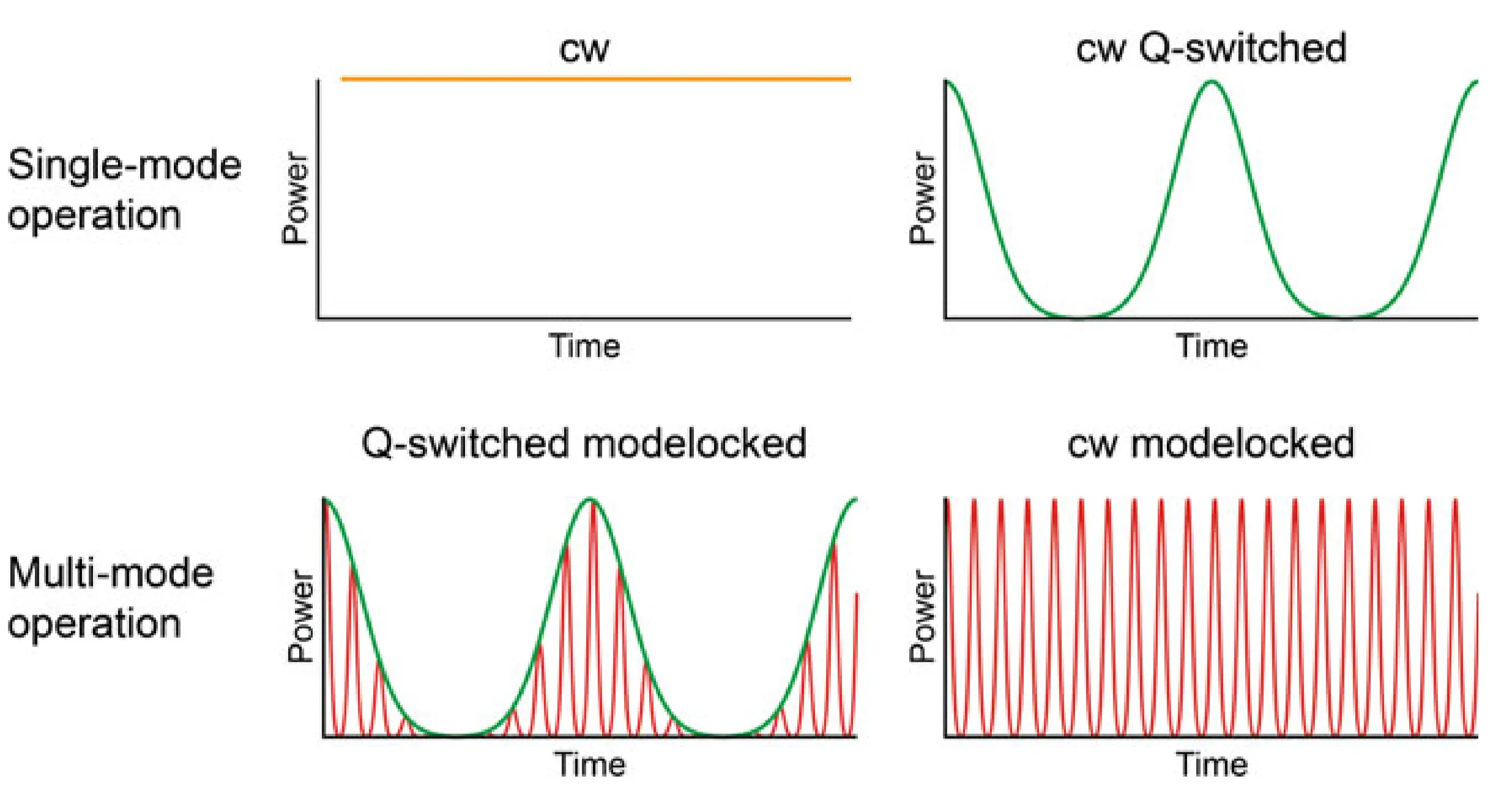
The individual pulse duration is controlled by the spectral envelope ${\tilde{E}}_{p} (ω)$ and its phase $\tilde{ϕ} (ω)$ , while the pulse-to-pulse spacing is fixed by the cavity roundtrip time.

Attachments/UltraFastLasers_Keller 67.webp|700

It is useful to keep three regimes separate:

Q-switching: the intracavity loss is changed slowly compared with the cavity roundtrip time. Energy builds up in the gain medium and is then dumped in a comparatively long pulse. The repetition rate is not the cavity axial-mode spacing.
Modelocking: the laser emits one or more pulses per cavity roundtrip. The pulse repetition rate is fixed by the roundtrip time, and the optical spectrum consists of phase-locked axial modes.
Q-switched modelocking: a short modelocked pulse train exists, but its envelope is modulated by slower Q-switched macropulses. This is usually an instability for lasers intended to run in steady modelocked operation.

For picosecond active modelocking, the slowly-varying-envelope approximation is usually safe. For few-cycle passive modelocking, the position of the carrier field under the envelope becomes important; this is the carrier-envelope offset discussed in chapter 12.

This distinction also explains why active modelocking is historically important but not usually the final source for high-harmonic generation. Active modelocking can produce a stable and electronically synchronised pulse train, but the pulses are typically too long and have too little peak electric field for efficient HHG. Attosecond experiments usually need the additional pulse shortening, dispersion control, nonlinear broadening, and CEO control discussed in the later passive modelocking and comb chapters.

6.2 Basic Principle of Active Modelocking

In active modelocking the laser contains an intracavity modulator driven by an external radio-frequency signal. The modulator changes the loss periodically with period $T_{R}$ or with a rational fraction of it. If exactly one pulse circulates in the cavity, the modulation is called fundamental active modelocking and the drive frequency is

f_{m} = f_{rep} = \frac{1}{T_{R}} .

For a linear standing-wave cavity, the modulator is usually placed close to an end mirror. Then the right- and left-propagating parts of the pulse pass the modulator at nearly the same modulation phase. If the modulator is placed at a more general position, the two passages see different phases and harmonic modelocking or unstable operation can be favoured.

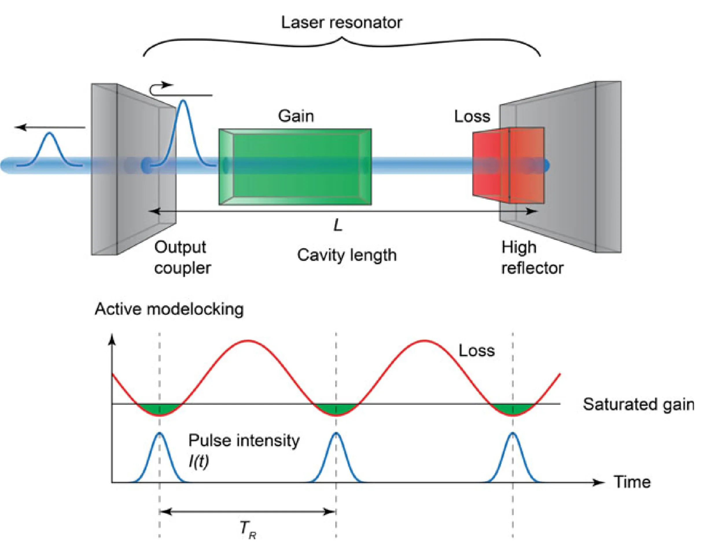
Attachments/UltraFastLasers_Keller 68.webp|700

The loss modulation can be expanded around its minimum as

l (t) = l_{0} + M [1 - \cos (Ω_{m} t)] \approx l_{0} + \frac{1}{2} M Ω_{m}^{2} t^{2},

where $Ω_{m} = 2 π f_{m}$ and $M$ describes the modulation strength. A pulse centred at the loss minimum experiences less loss than a broad pulse, so the modulator favours temporal shortening.

This shortening cannot continue indefinitely. Shorter pulses have broader spectra, and a real gain medium has a finite gain bandwidth. Frequencies far from the gain maximum experience less gain, so the gain medium acts as a spectral filter. In time-domain language, gain filtering broadens the pulse. Active modelocking without strong dispersion or nonlinearity is therefore a balance:

the time-dependent loss modulator narrows the pulse in time;
the finite gain bandwidth narrows the spectrum and therefore broadens the pulse in time.

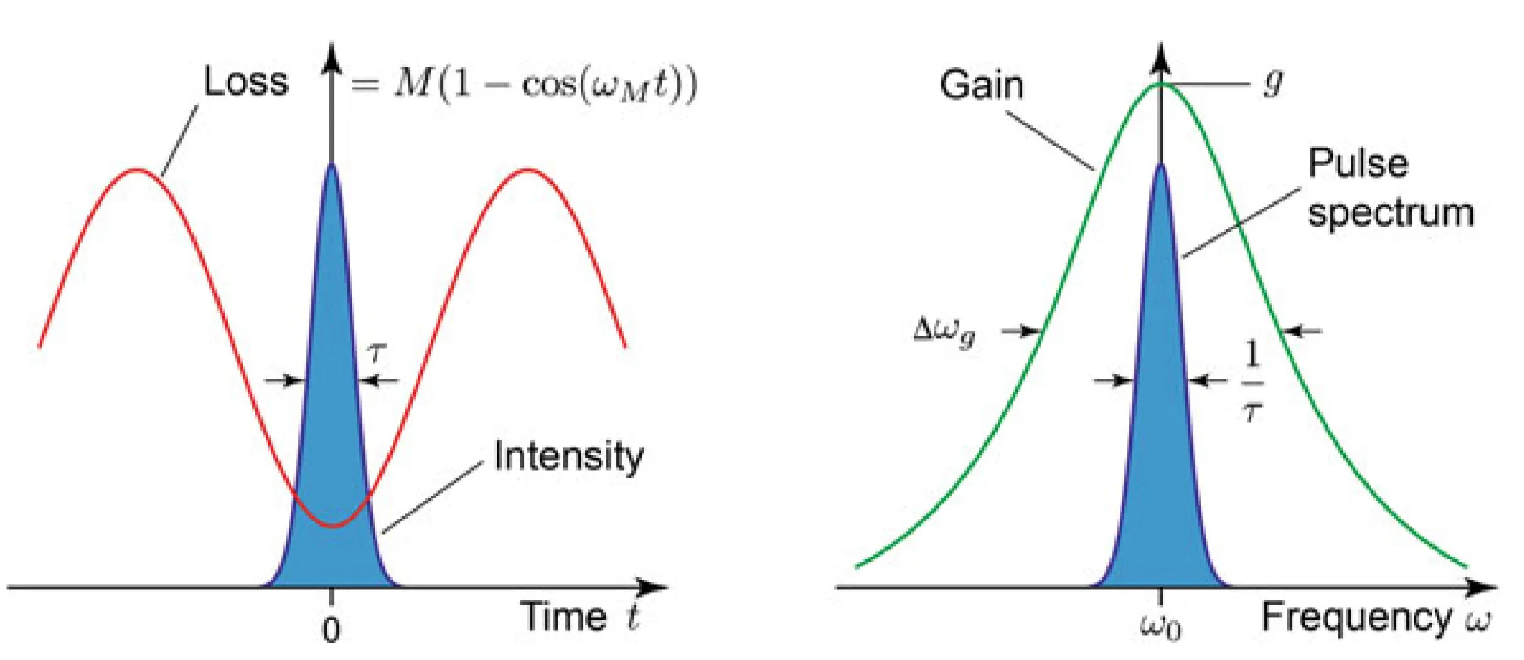
Attachments/UltraFastLasers_Keller 69.webp|700

The same idea can be viewed in the frequency domain. A sinusoidal modulation at the axial-mode spacing couples one axial mode to its neighbours. The modulation sidebands are phase coherent with the original field, so the modulator effectively seeds adjacent modes with a fixed phase relation. Repeating this process over many modes creates a phase-locked comb.

6.3 Optical Loss Modulators

Most active modelocked solid-state lasers use an acousto-optic modulator (AOM) or an electro-optic modulator (EOM). In both cases, the goal is not only to vary the loss but to vary it at a frequency phase-locked to the resonator roundtrip.

For an AOM, an acoustic wave creates a time-dependent refractive-index grating in a transparent medium. The optical beam is diffracted by this grating; if the laser uses the undiffracted beam, diffraction appears as a controllable loss. A standing acoustic wave can therefore produce a nearly sinusoidal loss modulation.

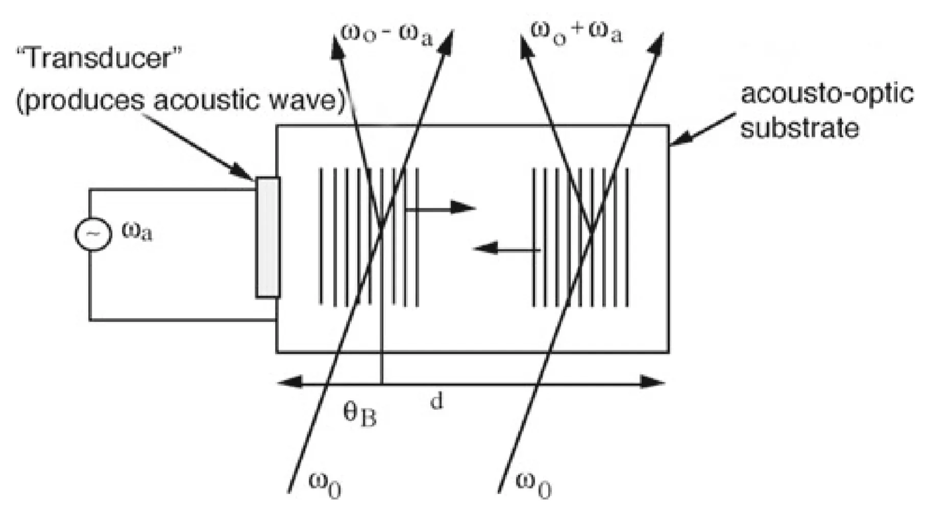
Attachments/UltraFastLasers_Keller 70.webp|700

If the acoustic wave has frequency $ω_{a}$ , a standing-wave intensity pattern modulates the refractive index at approximately $2 ω_{a}$ . The optical loss modulation is then adjusted such that its period matches the pulse roundtrip time. The modulation depth must be large enough to discriminate against light away from the preferred time slot, but excessive loss increases threshold and can destabilise the laser.

An EOM can also be used. It changes the refractive index through the electro-optic effect and can be turned into an amplitude modulator with polarisation optics. EOMs can be faster than AOMs, but in many solid-state laser systems AOMs are convenient because they provide direct amplitude modulation and can handle useful optical powers.

6.4 Active Modelocking Without SPM and GDD

The cleanest analytical model neglects both self-phase modulation and group-delay dispersion. In this limit, the relevant effects are saturated gain, finite gain bandwidth, constant loss, and time-dependent modulator loss.

The gain can be approximated by a parabola around the centre frequency:

g (ω) \approx g_{0} [1 - \frac{(ω - ω_{0})^{2}}{Ω_{g}^{2}}] .

In the time domain this produces a gain-filtering operator proportional to $\partial^{2} / \partial t^{2}$ , since multiplication by $(ω - ω_{0})^{2}$ in frequency corresponds to a second derivative in time.

A schematic Haus master equation for the pulse envelope $A (T, t)$ is then

T_{R} \frac{\partial A}{\partial T} = [g - l D_{g} \frac{\partial^{2}}{\partial t^{2}} - \frac{1}{2} M Ω_{m}^{2} t^{2}] A .

Here $t$ is the local time within one pulse, while $T$ counts the slow evolution over many cavity roundtrips. The terms have the following meaning:

$g - l$ is the net roundtrip gain.
$D_{g} \partial_{t}^{2}$ is the finite gain bandwidth written as a time-domain filtering term.
$- \frac{1}{2} M Ω_{m}^{2} t^{2}$ is the parabolic approximation to the modulator loss near its minimum.

This equation is mathematically similar to a harmonic-oscillator eigenvalue problem. The lowest-loss steady-state solution is Gaussian:

A (t) = A_{0} \exp (- \frac{t^{2}}{2 τ_{p}^{2}}) .

The exact pulse duration depends on the gain bandwidth and the modulation strength, but the scaling is the important part:

τ_{p} \propto {(\frac{D_{g}}{M Ω_{m}^{2}})}^{1 / 4} .

Thus stronger modulation shortens the pulse, while narrower gain bandwidth lengthens it. This fourth-root dependence is also a practical warning: improving the pulse duration by active modulation alone becomes inefficient.

The Gaussian solution also explains why active modelocking naturally produces picosecond rather than femtosecond pulses in many solid-state lasers. Without a strong nonlinear mechanism, pulse shortening is limited by the relatively gentle balance between a parabolic time gate and a finite spectral filter.

A useful way to remember this result is that active modelocking supplies an externally imposed clock, but not a strong self-compression mechanism. The RF modulation fixes the time slot in which light can survive. It does not by itself generate the octave-spanning spectra or sub- $10$ fs pulse envelopes needed for waveform-sensitive strong-field physics.

6.5 Adding SPM and GDD

When the pulse becomes shorter or the intracavity peak power becomes larger, the simple Gaussian model is no longer sufficient. Two additional effects become important:

SPM creates an intensity-dependent phase shift.
GDD creates a frequency-dependent delay.

Including these terms, the master equation takes the schematic form

T_{R} \frac{\partial A}{\partial T} = [g - l D_{g} \frac{\partial^{2}}{\partial t^{2}} - \frac{1}{2} M Ω_{m}^{2} t^{2} + i \frac{D_{2}}{2} \frac{\partial^{2}}{\partial t^{2}} + i γ | A |^{2}] A .

$D_{2}$ is the roundtrip group-delay dispersion and $γ$ is the roundtrip nonlinear phase coefficient. The last two terms are phase terms, but they still change the steady-state pulse because chirp changes how the pulse interacts with gain filtering and the modulator.

If SPM is present but GDD is negligible, the pulse acquires a nonlinear chirp but does not benefit from the soliton balance familiar from fibre propagation. The finite gain bandwidth then has to filter a broadened and chirped spectrum, which can limit stability.

If GDD and SPM have the right signs, the pulse can approach a soliton-like state. The intuitive condition is the same as for soliton propagation:

\frac{| D_{2} |}{τ_{p}^{2}} \sim γ P_{0},

where $P_{0}$ is the pulse peak power. In this regime dispersion and nonlinearity balance each other, while gain, loss, and the active modulator select the stable circulating pulse.

This is not yet the usual passive soliton modelocking discussed later, because the time gate is still imposed by an external modulator. Nevertheless, the same physical ingredients appear: gain filtering, dispersion, nonlinear phase, and loss discrimination.

In practice this means that the boundary between "active" and "passive" modelocking is not a boundary between linear and nonlinear physics. Active modelocking can still contain nonlinear phase and dispersion; it is called active because the primary pulse timing mechanism is externally driven. Passive modelocking is different because the pulse itself creates the loss discrimination.

6.6 Gain Broadening, Gain Saturation, and Synchronous Modelocking

The gain model matters. In a homogeneously broadened gain medium, all axial modes compete for the same inversion. Without a mechanism that enforces phase locking, this tends to favour single-mode operation. In an inhomogeneously broadened medium, different spectral parts can saturate somewhat independently, so multimode operation can be easier. However, multimode operation alone is not modelocking; the phases still have to be locked.

The gain saturation time scale also matters. Many solid-state laser gain media have upper-state lifetimes much longer than the pulse period, so the gain mostly responds to the average intracavity power. In that case, active modelocking is dominated by the externally imposed loss gate. If the gain can respond within or between pulses, dynamic gain saturation can contribute an additional shaping mechanism.

Synchronous modelocking is a related technique in which the gain, rather than the loss, is modulated by an external pulse train. This can be achieved by pumping the laser with another modelocked laser. The pump pulse train must be synchronised to the cavity roundtrip:

T_{pump} \approx T_{R} .

The gain then exists only in a narrow time window, so the laser preferentially supports a pulse that overlaps that window. The principle is similar to active loss modulation, but the time gate appears as gain enhancement instead of loss suppression.

In all forms of active modelocking, the central design requirement is phase coherence between the modulation and the cavity. If the drive frequency is detuned from the cavity roundtrip frequency, the pulse arrives progressively earlier or later relative to the modulation minimum. Small detunings can shift or chirp the steady-state pulse; large detunings prevent stable modelocking.