Table of Contents

5.1 Rate Equations for the Ideal Four-Level System
5.2 Relaxation Oscillations

5 Laser Rate Equations and Relaxation Oscillations

This chapter builds on the assumption that the reader is familiar with how lasers operate. Most modern lasers are diode-pumped solid-state lasers, typically pumped by high-power semiconductor diode arrays or bars. Since the individual diodes in such an array are not mutually coupled, the spatial coherence of the emitted pump beam is limited. Nevertheless, they are significantly brighter than flashlamps. More importantly, their much narrower spectral emission allows them to be tuned directly into an absorption line of the solid-state gain medium. This results in more efficient pump absorption and reduced thermal loading, especially when the pump photon energy is close to the upper laser level energy. A primary advantage of diode-pumped solid-state lasers is their ability to convert low-cost, low-beam-quality optical power from high-power diode arrays into a near-diffraction-limited output beam with high efficiency.

As the following figure illustrates, one can distinguish between longitudinally and transversally pumped schemes:

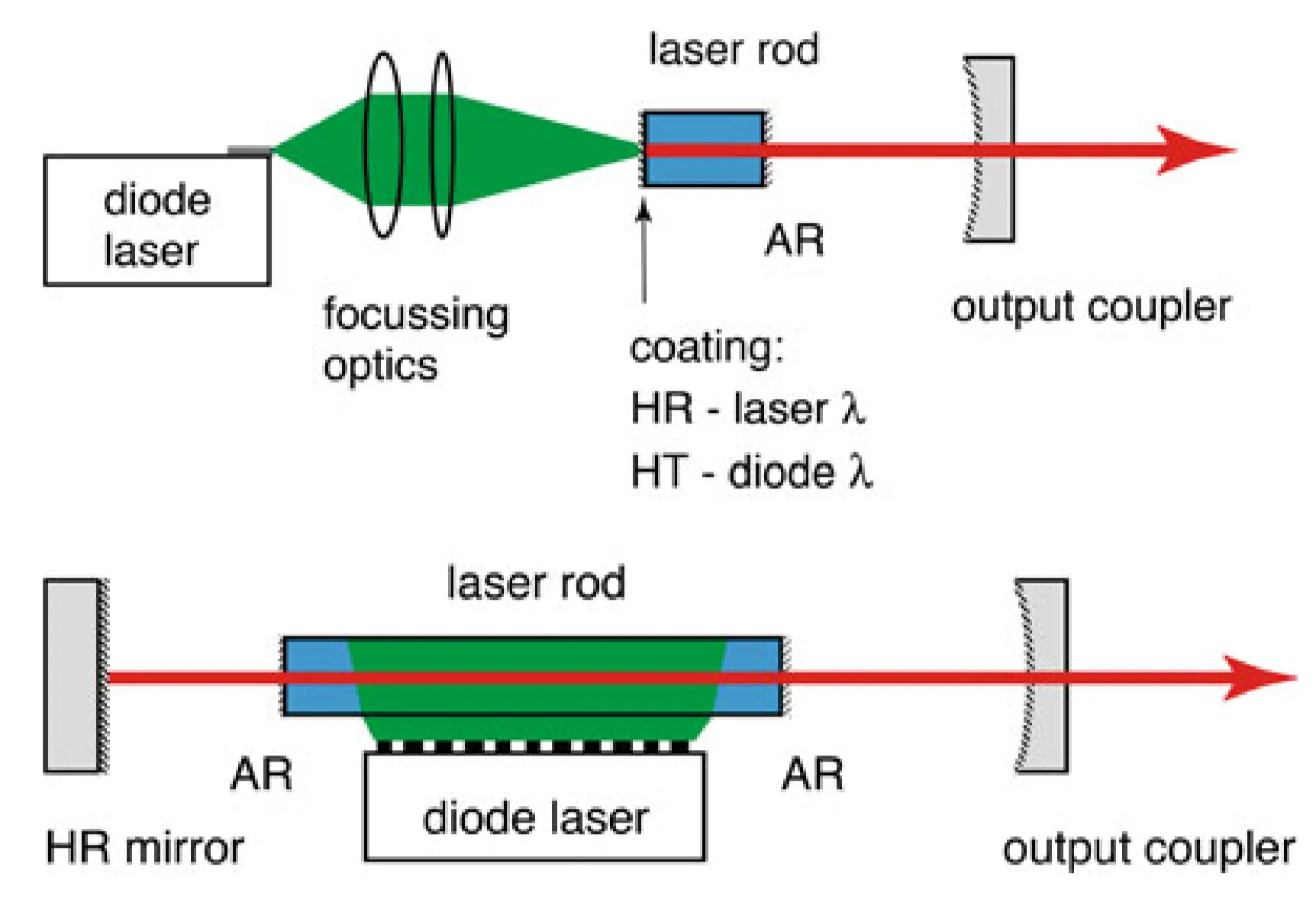
Attachments/UltraFastLasers_Keller 58.webp|700

Longitudinal pumping generally offers superior pumping efficiency in the low-power regime because the pump volume can be well matched to the laser mode volume within the laser crystal. For the laser crystal itself, a distinction is made by the type of lasing transition. Most often, three-level and four-level systems are employed, as shown below:

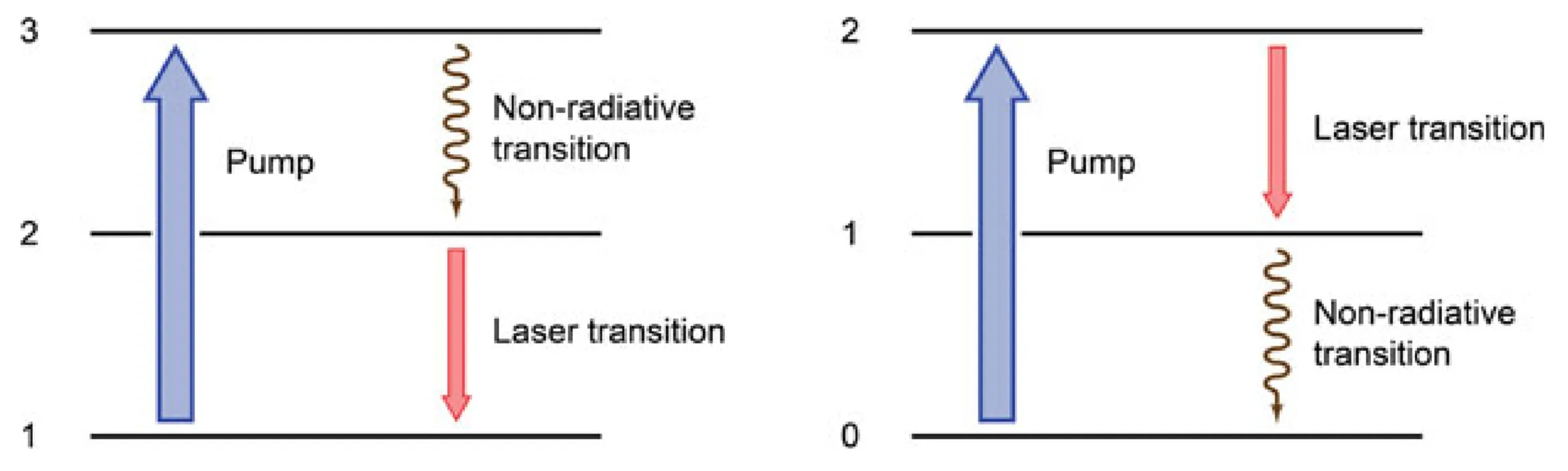
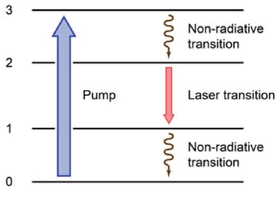
Attachments/UltraFastLasers_Keller 59.webp|700

The four-level system represents an ideal case, although careful design can also yield excellent performance from a three-level laser. The following discussion will focus on the ideal four-level laser system, for which the three-level system requires some modification. This is not discussed further here but is treated in my other notes here.

5.1 Rate Equations for the Ideal Four-Level System

We consider a homogeneously broadened laser medium within a linear resonator, which supports standing waves inside the cavity. The saturated gain coefficient is described by

g = \frac{g_{0}}{1 + 2 I / I_{sat}}

where $g_{0}$ is the small-signal gain coefficient and $I$ is the intra-cavity intensity. The factor of 2 in the denominator arises from spatial hole burning in a standing-wave cavity. The saturation intensity for a four-level laser material is $I_{sat} = \frac{h ν}{σ τ_{L}}$ , with $σ$ being the gain cross-section and $τ_{L}$ the spontaneous lifetime of the upper laser level. With increasing intensity inside the resonator, $g$ decreases ('saturates') until a steady-state intensity is reached where gain equals loss, $g (t \to \infty) = l$ . Here, $l$ represents the total resonator losses, including output coupling. The steady-state intensity $I_{s}$ is found by setting $g = l$ :

I_{s} = \frac{I_{sat}}{2} (\frac{g_{0}}{l} - 1)

Unless stated otherwise, we use amplitude gain and loss coefficients. The rate equations for the photon number inside the cavity laser mode, $n$ , and the population inversion, $N$ , are

\begin{aligned} \frac{d n}{d t} = K (n + 1) N - γ_{c} n \\ \frac{d N}{d t} = R_{p} - K n N - γ_{L} N \end{aligned}

where $K$ is the coupling constant, $R_{p}$ is the pumping rate into the upper laser level, $γ_{L} = 1 / τ_{L}$ is the spontaneous decay rate of the inversion (atomic decay rate), and $γ_{c} = 1 / τ_{c}$ is the cavity decay rate. Each term corresponds to a specific process:

\begin{aligned} Stimulated emission: & K n N \\ Spontaneous emission into the laser mode: & K N \end{aligned}

Stimulated emission appears in both equations with opposite signs, signifying that a decrease in inversion leads to an increase in the photon number. The stimulated transition probability $W^{stim}$ for $N$ inverted atoms is given by

W^{stim} = N (K n) = K n N = \frac{I}{h ν} σ N

where $σ$ is the gain cross-section of the laser material.

5.1.1 Steady-State Solution

Steady-state is defined by a constant photon number $n_{s}$ and a constant inversion $N_{s}$ :

\frac{d n_{s}}{d t} = 0 and \frac{d N_{s}}{d t} = 0

This simplifies the rate equations to

\begin{aligned} K (n_{s} + 1) N_{s} - γ_{c} n_{s} = 0 \\ R_{p} - K n_{s} N_{s} - γ_{L} N_{s} = 0 \end{aligned}

From the first equation, we can solve for the steady-state inversion $N_{s}$ and photon number $n_{s}$ . Introducing the threshold inversion $N_{th} = γ_{c} / K$ , the inversion required to achieve gain equal to cavity losses, we find

N_{s} = N_{th} \frac{n_{s}}{n_{s} + 1} and n_{s} = \frac{N_{s}}{N_{th} - N_{s}}

From the second equation, we find an alternative expression for the inversion:

N_{s} = \frac{R_{p}}{K n_{s} + γ_{L}} = \frac{R_{p} τ_{L}}{1 + K τ_{L} n_{s}}

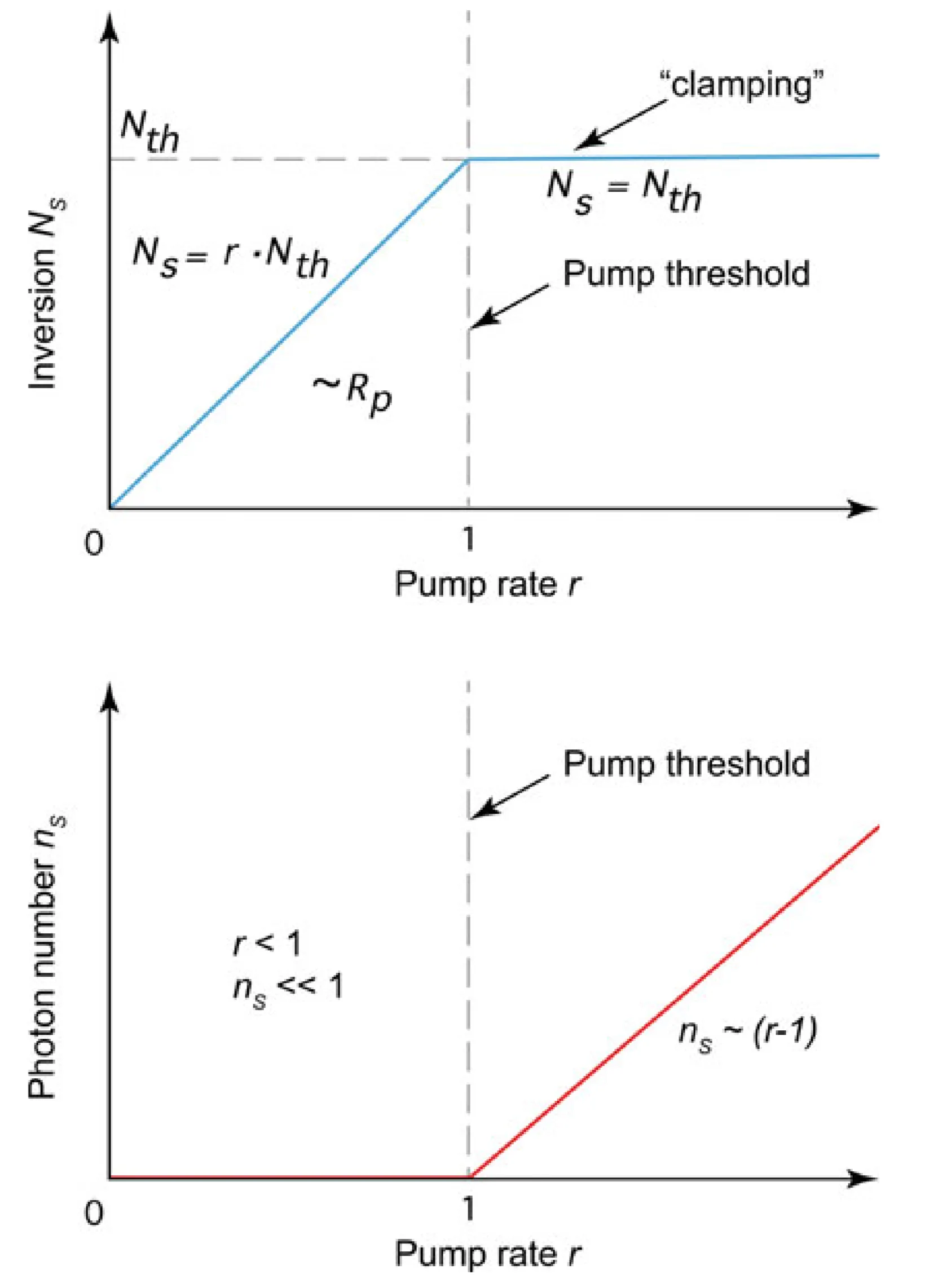
We now define the threshold pumping rate $R_{p, th}$ as the rate required to reach the threshold inversion $N_{th}$ in the absence of laser oscillation ( $n_{s} \to 0$ ). From the equation above, this gives $N_{th} = R_{p, th} τ_{L}$ , so

R_{p, th} = \frac{N_{th}}{τ_{L}}

It is convenient to introduce the normalized pumping rate as the ratio of the pump rate to the threshold pump rate:

r \equiv \frac{R_{p}}{R_{p, th}}

For a pump rate below threshold ( $r < 1$ ), the photon number $n_{s}$ is very small. The inversion thus grows linearly with the pump rate:

N_{s} \approx R_{p} τ_{L} = r R_{p, th} τ_{L} = r N_{th} for n_{s} ≪ 1 / (K τ_{L}) and r < 1

Above threshold ( $r > 1$ ), the steady-state photon number $n_{s}$ becomes larger by many orders of magnitude, such that $n_{s} ≫ 1$ . In this regime, the expression $N_{s} = N_{th} \frac{n_{s}}{n_{s} + 1}$ shows that the inversion becomes fixed, or clamped, at the threshold value:

N_{s} \approx N_{th} for n_{s} ≫ 1 and r > 1

Therefore, above threshold, the inversion remains constant even if the laser is pumped harder. We can summarise the two distinct behaviours:

\begin{aligned} Below threshold r < 1 : & {\begin{matrix} n_{s} = \frac{r}{1 - r} \\ N_{s} \approx r N_{th} \end{matrix} \\ Above threshold r > 1 : & {\begin{matrix} n_{s} \approx \frac{τ_{c}}{τ_{L}} N_{th} (r - 1) = \frac{γ_{L}}{K} (r - 1) \\ N_{s} \approx N_{th} = \frac{γ_{c}}{K} \end{matrix} \end{aligned}

This behaviour is illustrated in the following figure:

Attachments/UltraFastLasers_Keller 61.webp|700

5.1.2 Gain-Saturation

The roundtrip amplitude gain in a linear cavity with a gain medium of length $L_{g}$ is $2 g$ , where $g = \frac{N_{s}}{V} σ L_{g}$ is the single-pass amplitude gain. Here, $N_{s} / V$ is the inversion density for a given mode volume $V$ . Substituting the steady-state inversion $N_{s}$ , we get

g = \frac{R_{p} τ_{L} σ L_{g}}{V (1 + K τ_{L} n_{s})}

Comparing this with the initial expression for saturated gain, $g = \frac{g_{0}}{1 + I / I_{sat}}$ , we can identify the small-signal (single-pass) gain $g_{0}$ and the saturation term:

g_{0} = L_{g} \frac{R_{p}}{V} τ_{L} σ and \frac{I}{I_{sat}} = K τ_{L} n_{s}

The small-signal gain coefficient $g_{0}$ depends on the laser material properties and the pump rate. Stronger pumping leads to a larger small-signal gain. Below the lasing threshold, the intracavity intensity is negligible, so the saturated gain is equal to the small-signal gain. At threshold, the gain exactly balances the losses, $g_{0} = l$ .

\begin{aligned} At threshold: & g_{0, th} = L_{g} \frac{R_{p, th}}{V} τ_{L} σ = l \\ Above threshold: & g_{0} = \frac{R_{p}}{R_{p, th}} g_{0, th} = r l \end{aligned}

This relationship is shown in the following figure:

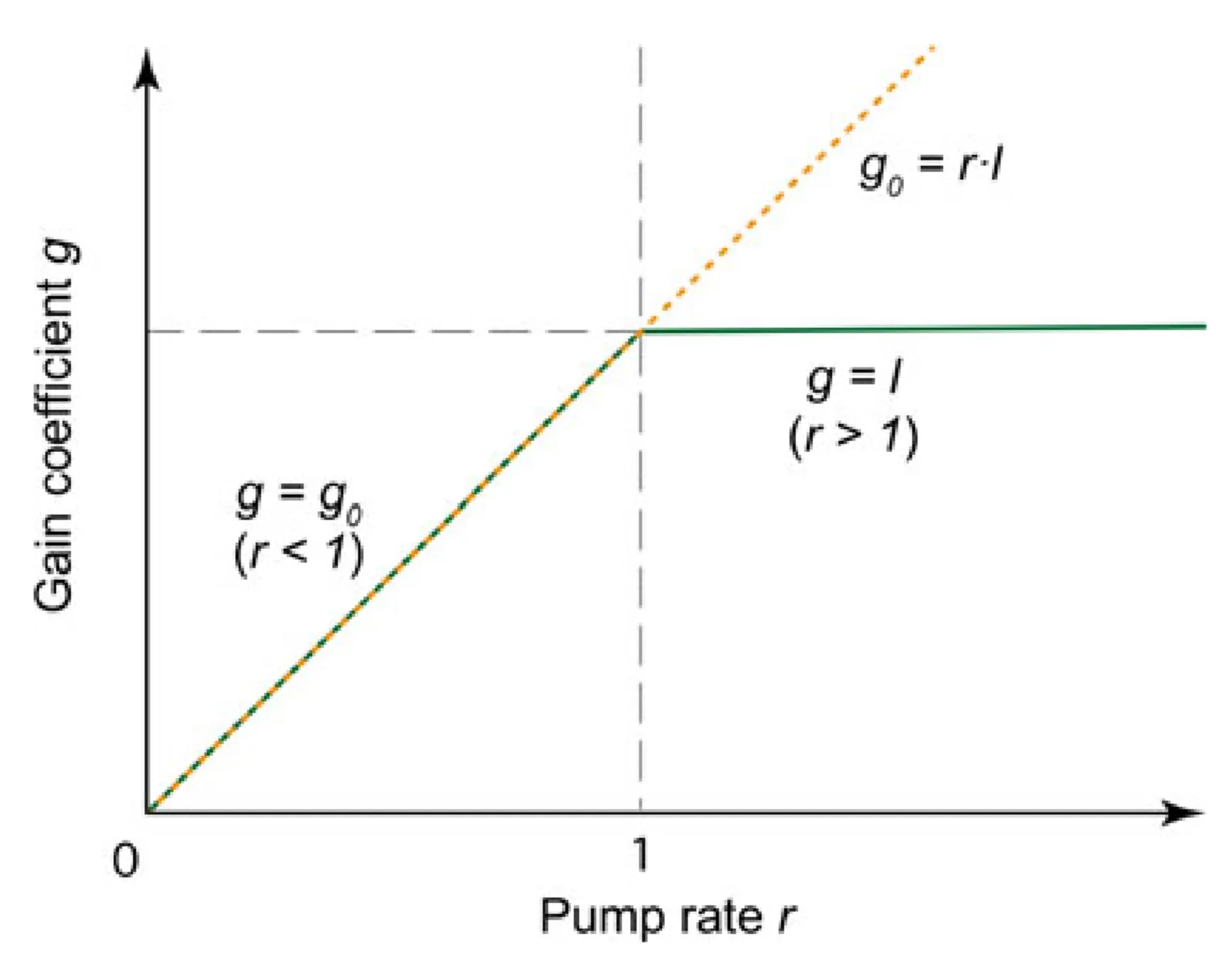
Attachments/UltraFastLasers_Keller 62.webp|700

Above threshold, inversion clamping ensures that each additional absorbed pump photon is converted into a photon via stimulated emission. Consequently, the output power increases linearly with pump power.

5.2 Relaxation Oscillations

As before, we consider the ideal four-level system. If the laser is briefly disturbed from its steady state, the photon number and inversion will deviate from their equilibrium values. It then takes a characteristic time to return to steady state. We can analyse this by linearising the rate equations for small perturbations, $δ n (t)$ and $δ N (t)$ , around the steady-state values:

\begin{aligned} n (t) = n_{s} + δ n (t) & with & δ n (t) ≪ n_{s} \\ N (t) = N_{s} + δ N (t) & with & δ N (t) ≪ N_{s} \end{aligned}

We consider small perturbations while the laser operates above threshold ( $n_{s} ≫ 1$ ), allowing us to neglect the spontaneous emission term $K N$ in the photon rate equation. Substituting the perturbed forms into the rate equations yields a set of linear differential equations for the perturbations. For the photon number:

\begin{aligned} \frac{d δ n}{d t} & = K (N_{s} + δ N) (n_{s} + δ n) - γ_{c} (n_{s} + δ n) \\ \approx K N_{s} n_{s} + K N_{s} δ n + K n_{s} δ N - γ_{c} n_{s} - γ_{c} δ n \end{aligned}

Using the steady-state conditions $K N_{s} n_{s} \approx γ_{c} n_{s}$ and $K N_{s} \approx γ_{c}$ , the equation simplifies to

\frac{d δ n}{d t} = K n_{s} δ N = γ_{L} (r - 1) δ N

Similarly for the inversion:

\begin{aligned} \frac{d δ N}{d t} & = R_{p} - K (N_{s} + δ N) (n_{s} + δ n) - γ_{L} (N_{s} + δ N) \\ \approx (R_{p} - K N_{s} n_{s} - γ_{L} N_{s}) - K N_{s} δ n - K n_{s} δ N - γ_{L} δ N \end{aligned}

The terms in the parenthesis sum to zero in steady state. This leaves

\frac{d δ N}{d t} = - K N_{s} δ n - (K n_{s} + γ_{L}) δ N

Using the above-threshold relations $K N_{s} \approx γ_{c}$ and $K n_{s} + γ_{L} = γ_{L} (r - 1) + γ_{L} = r γ_{L}$ , we obtain

\frac{d δ N}{d t} = - γ_{c} δ n - r γ_{L} δ N

5.2.1 Ansatz for Solutions After Perturbations

If the perturbation is short-lived, we expect the system to return to equilibrium. We thus propose an exponential ansatz for the perturbations:

δ n (t) \sim e^{s t} and δ N (t) \sim e^{s t}

For a stable laser, the real part of $s$ must be negative. Inserting this ansatz into the linearised rate equations yields a characteristic equation for $s$ : $s^{2} + r γ_{L} s + γ_{L} γ_{c} (r - 1) = 0$ . The solutions are

s_{1, 2} = - \frac{r γ_{L}}{2} \pm \sqrt{{(\frac{r γ_{L}}{2})}^{2} - γ_{L} γ_{c} (r - 1)}

The nature of the solution depends on the value of the discriminant.

Over-Critically Damped Laser
If the discriminant is positive, $s$ is real, and the system returns to steady-state without oscillations. This is typical for gas lasers, where the condition is

{(\frac{r γ_{L}}{2})}^{2} > γ_{L} γ_{c} (r - 1) ⟹ \frac{r γ_{L}}{4} > γ_{c} \frac{r - 1}{r}

In the limit where the stimulated decay rate is much larger than the cavity decay rate ( $r γ_{L} ≫ γ_{c}$ ), the two decay rates are approximately

s_{1} \approx - r γ_{L} and s_{2} \approx - γ_{c} \frac{r - 1}{r}

The system is called over-critically damped. After a perturbation, the laser returns to its steady state on timescales governed by the cavity photon lifetime and the stimulated lifetime of the laser level.

Under-Critically Damped Laser
If the discriminant is negative, $s$ is complex, leading to damped relaxation oscillations. This is typical for solid-state lasers, corresponding to the case

{(\frac{r γ_{L}}{2})}^{2} < γ_{L} γ_{c} (r - 1) ⟹ \frac{r γ_{L}}{4} < γ_{c} \frac{r - 1}{r}

The solution for $s$ is then

s_{1, 2} = - \frac{r γ_{L}}{2} \pm i \sqrt{γ_{L} γ_{c} (r - 1) - {(\frac{r γ_{L}}{2})}^{2}}

The solution for the photon number perturbation takes the form of a damped sinusoid:

δ n (t) = n_{1} e^{- γ_{relax} t} \cos (ω_{relax} t)

The real part of $s$ is the damping rate of the relaxation oscillation,

γ_{relax} = \frac{r γ_{L}}{2}

while the imaginary part of $s$ is the relaxation oscillation angular frequency,

ω_{relax} = \sqrt{γ_{L} γ_{c} (r - 1) - {(\frac{r γ_{L}}{2})}^{2}}

For many solid-state lasers, the cavity decay rate is much larger than the stimulated decay rate ( $γ_{c} ≫ r γ_{L}$ ). The frequency $f_{relax} = ω_{relax} / 2 π$ can be approximated as

f_{relax} \approx \frac{1}{2 π} \sqrt{γ_{L} γ_{c} (r - 1)} = \frac{1}{2 π} \sqrt{\frac{r - 1}{τ_{L} τ_{c}}} = \frac{1}{2 π} \sqrt{\frac{1}{τ_{stim} τ_{c}}}

Here, we defined the stimulated lifetime $τ_{stim} = τ_{L} / (r - 1)$ . Relaxation oscillations can be measured with a fast photodiode and a microwave spectrum analyser, appearing as a peak in the laser's intensity noise spectrum.

Attachments/UltraFastLasers_Keller 63.webp|700

The relaxation frequency increases with the pump power (since $r$ increases), and the strength of the relative intensity fluctuations decreases with increasing pump power, as

\frac{Δ P_{relax}}{P} \sim \frac{1}{γ_{relax}} = \frac{2}{r γ_{L}}

Therefore, the relative noise strength decreases for higher pump powers and shorter upper-state lifetimes.

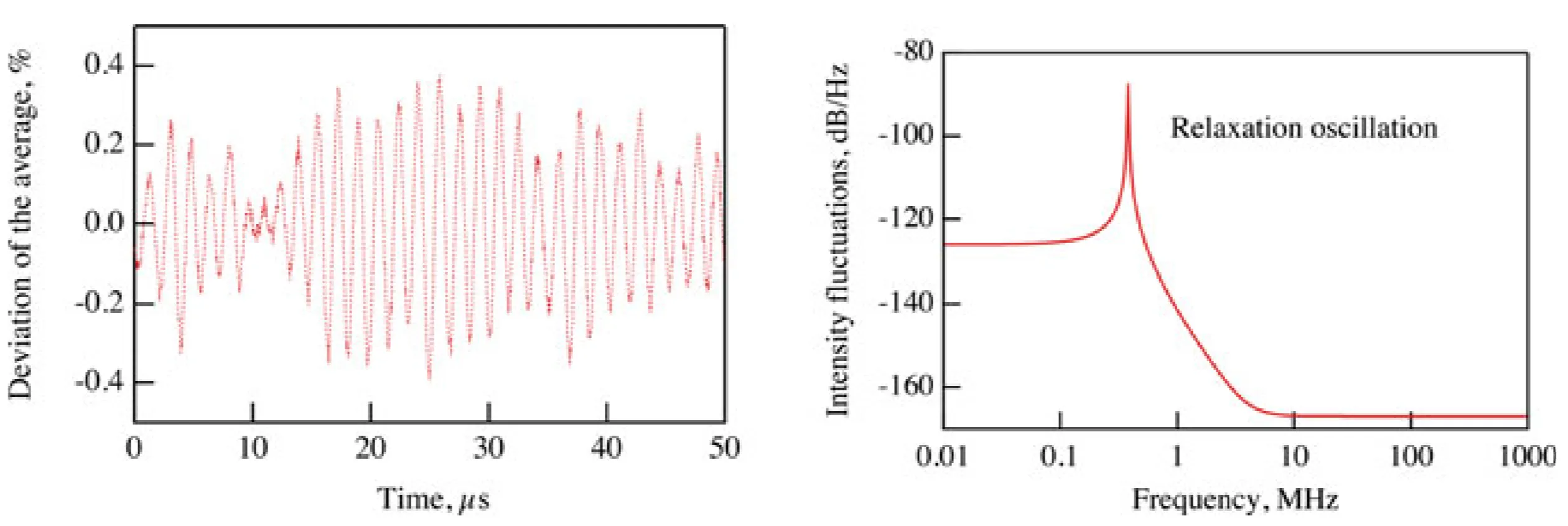
5.2.2 Measurement of the Small-Signal Gain

Relaxation oscillations provide a simple method to determine the small-signal gain $g_{0}$ of CW solid-state lasers. For lasers with high small-signal gain, such as diode-pumped solid-state lasers, measuring the lasing threshold to infer gain can be inaccurate. The small-signal gain is a fundamental parameter for laser design, influencing the choice of output coupler, predicting Q-switched laser performance, and affecting the dynamics of passively modelocked lasers.

For typical solid-state lasers like Nd:YAG, the upper-state lifetime $τ_{L}$ is hundreds of microseconds, much longer than the cavity lifetime $τ_{c}$ , which is typically tens to hundreds of nanoseconds. The approximation $r γ_{L} ≪ γ_{c}$ is therefore valid if the laser is not pumped excessively far above threshold. The relaxation oscillation frequency is then

f_{relax} \approx \frac{1}{2 π} \sqrt{\frac{r - 1}{τ_{L} τ_{c}}}

We can express the parameters in terms of measurable quantities. Using $r = g_{0} / l$ and the cavity lifetime $τ_{c} = T_{R} / (2 l)$ , where $T_{R}$ is the roundtrip time and $2 l$ is the roundtrip intensity loss, we get

f_{relax} \approx \frac{1}{2 π} \sqrt{\frac{(g_{0} / l) - 1}{τ_{L} (T_{R} / 2 l)}} = \frac{1}{2 π} \sqrt{\frac{2 (g_{0} - l)}{τ_{L} T_{R}}}

For high-gain lasers where $g_{0} ≫ l$ , the relaxation frequency becomes largely independent of the cavity loss and scales with the pump power:

f_{relax} \sim \sqrt{g_{0}} \sim \sqrt{P_{pump}}

By rearranging the formula, we can solve for the roundtrip small-signal gain $2 g_{0}$ :

2 g_{0} \approx 4 π^{2} τ_{L} T_{R} f_{relax}^{2} + 2 l

This relation allows for an accurate determination of the small-signal gain by measuring the relaxation oscillation frequency, the cavity roundtrip time, the total losses, and knowing the upper-state lifetime of the gain medium.