Jump back to chapter selection.

Table of Contents

2.1 Wave Equation in the Spectral Domain: Helmholtz Equation
2.2 Linear vs Nonlinear Wave Propagation
2.3 Ultrafast Pulses
2.4 Linear pulse Propagation in a Dispersive Material

2 Linear Pulse Propagation

In Chapter 1 we have seen that a monochromatic plane wave extends infinitely in space and time. To obtain a limited wave packet in time (a pulse), different plane waves with different wavelengths need to be superposed:

Attachments/UltraFastLasers_Keller 6.webp|700

In the visible spectrum, different wavelengths correspond to different colours. This has important implications: A laser pulse can never be single-coloured (monochromatic) and must differ from the monochromatic light of a continuous-wave (CW) laser. The more frequency components a pulse contains, the broader its spectrum is (by definition) and the shorter the pulse can be.

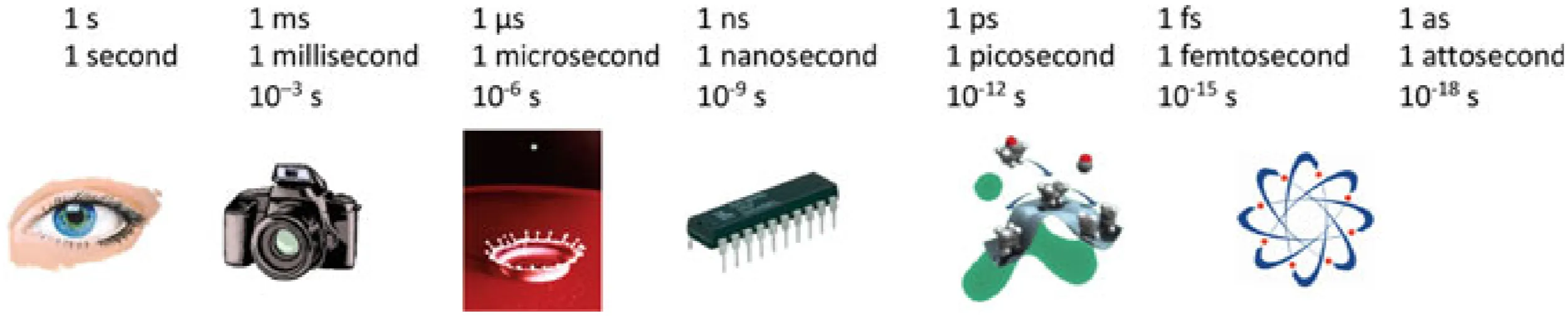
Before diving deeper into this topic, it is important to recall some orders of magnitude:

Attachments/UltraFastLasers_Keller 7.webp|700

Our eyes can only distinguish movements on timescales longer/slower than about $100 ms$ . Mechanical shutters determining the exposure time in photography are limited to about $1 ms$ . Any movements occurring faster than that will smear out on a photograph and will result in a blurry image. However, using strobe photography, it is possible to achieve exposure times as short as $1 μ s$ . With strobe photography, short light flashes started to become important for time-resolved measurements. Lasers are relevant here because we can generate much shorter flashes of light with lasers than with electrically switched light bulbs.

Today we can generate pulses as short as a few femtoseconds in the visible and near-infrared wavelength regimes directly from a laser. This is much faster than any electronic switching speed. For instance, in the nanosecond region, we find typical computer switching elements, and the fastest commercial microwave sampling oscilloscopes have a time resolution of around one picosecond.

It is good practice to remember these orders of magnitude!

2.1 Wave Equation in the Spectral Domain: Helmholtz Equation

We know that any function can be expanded in terms of a complete set of orthogonal functions. Examples of this are Fourier series and Fourier integrals. A Fourier transform decomposes an arbitrary function of time into its harmonic frequency components. The inverse Fourier transform does the opposite and constructs an arbitrary function of time as a superposition of harmonic functions of time with different frequencies:

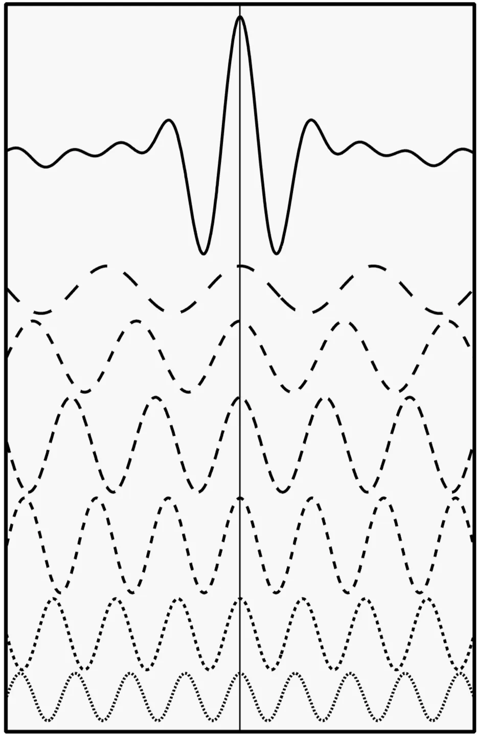
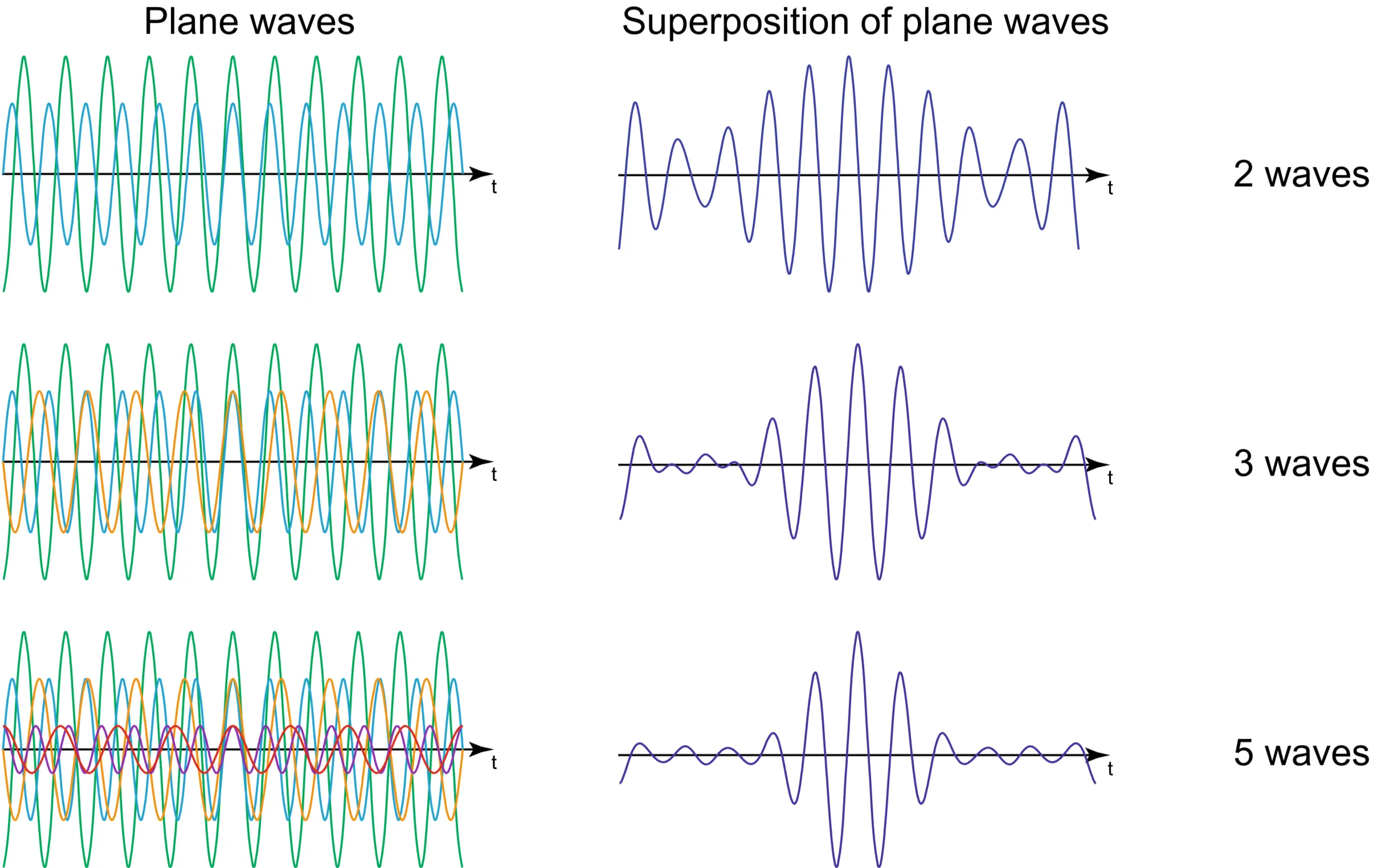
Attachments/UltraFastLasers_Keller 8.webp|700

This is a powerful tool for describing ultrashort pulses, since the harmonic components have the physical meaning of plane waves with different frequencies. A light pulse can be formed by a superposition of plane waves with different (possibly discrete) frequencies at a fixed position in space:

Attachments/UltraFastLasers_Keller 9.webp|700

The more waves are superposed, the shorter the pulse can be. If these frequencies are discrete and equally spaced, the superposition is not just one pulse, but a periodic pulse train with period $T_{rep} = 2 π / Δ ω$ , where $Δ ω$ is the constant frequency spacing in the example figure.

We will follow this convention for our Fourier transform $F$ and its inverse $F^{- 1}$ :

\begin{aligned} E (z, ω) \equiv F [E (z, t)] = \int_{- \infty}^{\infty} E (z, t) e^{- i ω t} d t, \\ E (z, t) = F^{- 1} [E (z, ω)] = \frac{1}{2 π} \int_{- \infty}^{\infty} E (z, ω) e^{+ i ω t} d ω, \end{aligned}

where we write the complex scalar electric field of an electromagnetic plane wave as:

E (z, t) = E_{0} e^{i (ω t - k z)} .

Regarding the constant $1 / (2 π)$ , we have chosen an asymmetric Fourier transform convention. This choice is common, particularly when relating spectra measured as a function of frequency $f$ to angular frequency $ω$ . We will subsequently make use of some useful operator correspondences derived from these definitions:

F^{- 1} {i ω E (z, ω)} = \frac{\partial}{\partial t} E (z, t) .

This leads to the abbreviated correspondence: $\frac{\partial}{\partial t} \leftrightarrow i ω$ , or $ω \leftrightarrow - i \frac{\partial}{\partial t}$ when moving from frequency domain to time domain operations. For higher derivatives, we have:

ω ⟺ - i \frac{\partial}{\partial t}, ω^{2} ⟺ {(- i \frac{\partial}{\partial t})}^{2} = - \frac{\partial^{2}}{\partial t^{2}}, ω^{3} ⟺ {(- i \frac{\partial}{\partial t})}^{3} = i \frac{\partial^{3}}{\partial t^{3}} .

Derivation
We start with the wave equation including a polarisation term $P$ :

\nabla^{2} E - \frac{1}{c^{2}} \frac{\partial^{2}}{\partial t^{2}} E = μ_{0} \frac{\partial^{2}}{\partial t^{2}} P .

Considering propagation in one dimension ( $z$ ) and using the relation for the second-order time derivative $\partial^{2} / \partial t^{2} \leftrightarrow - ω^{2}$ , we transform the scalar version of this equation to the spectral domain as:

\frac{\partial^{2} E (z, ω)}{\partial z^{2}} + \frac{ω^{2}}{c^{2}} E (z, ω) = - μ_{0} ω^{2} P (z, ω) .

For a linear, isotropic medium, the polarisation in the frequency domain is $P (z, ω) = ε_{0} χ (ω) E (z, ω)$ . Using the relative permittivity $ε_{r} (ω) = 1 + χ (ω)$ , we have $P (z, ω) = ε_{0} (ε_{r} (ω) - 1) E (z, ω)$ . Substituting this into the spectral wave equation and rearranging (using $c^{2} = 1 / (ε_{0} μ_{0})$ ) gives:

\frac{\partial^{2} E (z, ω)}{\partial z^{2}} + \frac{ω^{2}}{c^{2}} ε_{r} (ω) E (z, ω) = 0.

With the definition of the wave number in the medium $k_{n} (ω) = \frac{ω}{c} n (ω)$ and $n (ω) = \sqrt{ε_{r} (ω)}$ (assuming non-magnetic media, $μ_{r} = 1$ ), we find the one-dimensional Helmholtz equation:

\frac{\partial^{2} E (z, ω)}{\partial z^{2}} + {[k_{n} (ω)]}^{2} E (z, ω) = 0.

This is the wave equation in the spectral domain for a dispersive linear medium with an arbitrary dispersion relation $n (ω)$ (and $μ_{r} = 1$ ). It is easy to verify that its general solution is:

E (z, ω) = E_{0}^{+} (ω) e^{- i k_{n} (ω) z} + E_{0}^{-} (ω) e^{+ i k_{n} (ω) z},

which is analogous to the time-independent Schrödinger equation for a free particle. Hence, the discussion on laser pulse propagation also applies to the propagation of quantum mechanical wave packets.

2.2 Linear vs Nonlinear Wave Propagation

In linear optics, the wave equation is linear, meaning that the electric and magnetic fields and their derivatives appear only to the first order. Therefore, the superposition principle is valid, such that linear combinations of individual solutions ( $E_{i}, H_{i}$ ) are solutions as well:

E_{total} = \sum_{i} a_{i} E_{i} and H_{total} = \sum_{i} a_{i} H_{i} .

(Here we assume $a_{i} = b_{i}$ as $E_{i}$ and $H_{i}$ for a given mode are uniquely related).
Furthermore, the superposition principle is not generally valid for intensities:

I_{total} \neq \sum_{i} I_{i},

since, for instance, $| E_{1} + E_{2} |^{2} \neq | E_{1} |^{2} + | E_{2} |^{2}$ if there is interference. However, it will hold even for intensities if the electromagnetic fields do not satisfy the conditions for interference, for instance when they are polarised perpendicular to each other, or when two waves are fully incoherent.

2.2.1 Linear System Theory

This topic is covered briefly here to the extent required. For a more detailed treatment, I invite you to read my notes on Signals and Systems.

In a linear system, we can directly connect the input signal to the output signal by considering linearity:

E_{in 1} \overset{linear system}{\to} E_{out 1} ⟹ a E_{in 1} \overset{linear system}{\to} a E_{out 1},

and the fact that the superposition principle is valid:

\begin{array}{l} E_{in 1} \overset{linear system}{\to} E_{out 1} \\ E_{in 2} \overset{linear system}{\to} E_{out 2} \end{array}} ⟹ E_{in 1} + E_{in 2} \overset{linear system}{\to} E_{out 1} + E_{out 2} .

Examples include dispersive media (for field propagation), photodetectors (relating photocurrent output to incoming light power input, a linear power relationship), lens systems (for field transformations), and linear filters acting on stochastic processes. However, one must be careful: a photodetector's current output is typically linearly related to the input intensity (power), not directly to the input electric field for general linear field-to-field system theory.

In a linear system, we define the impulse response $h (t)$ : If the input is an infinitely short pulse $δ (t)$ (the Dirac delta function, called an impulse in system theory), the output is the function $h (t)$ . Knowing $h (t)$ is sufficient to find the output for any input $E_{in} (t)$ :

E_{out} (t) = \int_{- \infty}^{\infty} h (t^{'}) E_{in} (t - t^{'}) d t^{'} \equiv (h * E_{in}) (t) .

The symbol $*$ abbreviates convolution. In the spectral domain, the dynamics of a linear system are described by its transfer function $H (ω)$ (sometimes denoted $h (ω)$ ), which is the Fourier transform of $h (t)$ . The linear system response in the spectral domain is then given by simple multiplication:

E_{out} (ω) = H (ω) E_{in} (ω) .

The power spectral density $P_{E} (ω)$ of a signal $E (t)$ is given by:

P_{E} (ω) \equiv | E (ω) |^{2} .

Thus, $P_{in} (ω) = | E_{in} (ω) |^{2}$ and $P_{out} (ω) = | E_{out} (ω) |^{2}$ .
Analogously, for the system, $S_{H} (ω) \equiv | H (ω) |^{2}$ is the squared magnitude of the transfer function.
For a linear system, the relationship between input and output power spectra is:

P_{out} (ω) = S_{H} (ω) P_{in} (ω) .

From these considerations, it becomes clear why calculations in the spectral domain are often preferred: the complicated convolution in the time domain becomes a simple multiplication in the frequency domain.

We can use the transfer function $H (ω) = e^{- i k_{0} L_{d}}$ (where $k_{0} = ω / c$ ) for propagation over a distance $L_{d}$ in vacuum to find that the impulse response $h (t) = δ (t - L_{d} / c)$ . Then:

E_{out} (t) = \int_{- \infty}^{\infty} δ (t^{'} - \frac{L_{d}}{c}) E_{in} (t - t^{'}) d t^{'} = E_{in} (t - \frac{L_{d}}{c}) .

This implies that an arbitrary pulse $E_{in} (t)$ propagates in vacuum without changing its pulse shape, only experiencing a delay. This is no longer the case in a dispersive material, because the transfer function $H (ω) = e^{- i k_{n} (ω) L_{d}} = e^{- i ω n (ω) L_{d} / c}$ generally does not correspond to a simple time-shifted Dirac delta function for its impulse response $h (t)$ if $n (ω)$ is not constant.
A crucial conclusion for linear, lossless dispersive media is that $| H (ω) |^{2} = {| e^{- i k_{n} (ω) L_{d}} |}^{2} = 1$ (since $k_{n} (ω)$ is real for lossless media). Thus, $S_{H} (ω) = 1$ . This means the shape of the pulse power spectrum, $P_{E} (ω)$ , never changes during linear propagation in such a medium ( $P_{out} (ω) = P_{in} (ω)$ ). This is in stark contrast to nonlinear pulse propagation. Therefore, if the optical spectrum of a laser pulse changes in an experiment, it indicates the presence of some nonlinearity in the system.

2.3 Ultrafast Pulses

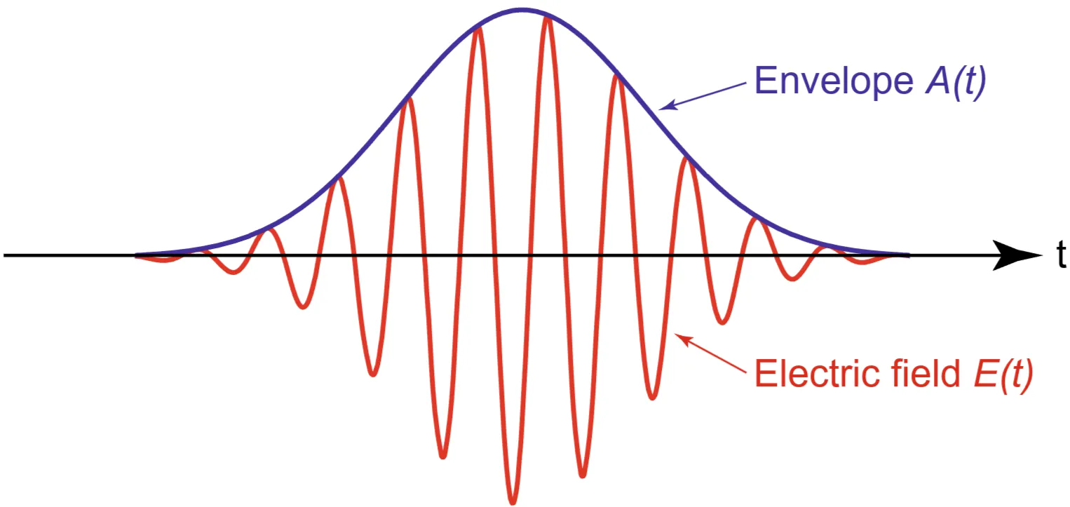
A coherent light pulse forms a wave packet of photons and can be described as a superposition of plane waves with different frequencies and phases at a fixed position in space. The shortest possible pulse duration for a given spectral amplitude distribution is obtained when the spectral phase is flat (constant) or linear with frequency (see section 2.3.2). For a pulse observed at a fixed position, we find its temporal profile via the inverse Fourier transform:

E (t) = \frac{1}{2 π} \int_{- \infty}^{\infty} E (ω) e^{i ω t} d ω .

The spectrum $E (ω)$ typically has a finite width $Δ ω_{0}$ (spectral bandwidth) centred around a carrier frequency $ω_{0}$ . For pulses significantly longer than one optical period ( $T_{0} = 2 π / ω_{0}$ ), we typically have $ω_{0} ≫ Δ ω_{0}$ . The exact shape and phase of $E (ω)$ determine the temporal shape of the light pulse $E (t)$ .

It is often useful to rewrite the prior equation by separating the carrier frequency. Replacing $ω$ with $ω_{0} + Δ ω$ (where $Δ ω = ω - ω_{0}$ is the frequency offset from the carrier) and integrating over $Δ ω$ :

E (t) = \frac{1}{2 π} \int_{- \infty}^{\infty} E (ω_{0} + Δ ω) e^{i (ω_{0} + Δ ω) t} d Δ ω = \frac{1}{2 π} e^{i ω_{0} t} \int_{- \infty}^{\infty} A_{spec} (Δ ω) e^{i Δ ω t} d Δ ω .

Here, $A_{spec} (Δ ω) = E (ω_{0} + Δ ω)$ is the frequency-shifted (baseband) spectrum. This implies that the time-domain field can be written as:

E (t) = A (t) e^{i ω_{0} t},

where

A (t) = \frac{1}{2 π} \int_{- \infty}^{\infty} A_{spec} (Δ ω) e^{i Δ ω t} d Δ ω

is called the complex pulse envelope. It describes the (generally slower) variation of the pulse's amplitude and phase relative to the fast carrier oscillation $e^{i ω_{0} t}$ .

Attachments/UltraFastLasers_Keller 10.webp|700

2.3.1 Time-Bandwidth Product

In laser physics, the laser pulse duration $τ_{p}$ is typically defined as the Full Width at Half Maximum (FWHM) of the time-dependent pulse intensity $I (t) \sim | E (t) |^{2} = | A (t) |^{2}$ . Analogously, the laser pulse spectral width $Δ f_{p}$ is normally defined as the FWHM of the spectral intensity (or power spectral density) $| E (ω) |^{2}$ (or $| E (f) |^{2}$ ).
The time-bandwidth product (TBP), $Δ f_{p} \cdot τ_{p}$ , has a minimum theoretical value that depends on the pulse shape. Some values are summarised below:

	$I (t)$ , where $x \equiv t / τ_{char}$	$τ_{p} / τ_{char}$	$Δ f_{p} \times τ_{p}$
Gaussian	$I (t) = e^{- x^{2}}$	$2 \sqrt{\ln 2}$	0.4413
Hyperbolic secant ( ${sech}^{2}$ )	$I (t) = {sech}^{2} x$	1.7627	0.3148
Rectangle	$I (t) = {\begin{cases} 1, & x \leq 1 / 2 \\ 0, & x > 1 / 2 \end{cases}$ (width $τ_{char}$ )	1	0.8859
Parabolic	$I (t) = {\begin{cases} 1 - x^{2}, & x \leq 1 \\ 0, & x > 1 \end{cases}$	$\sqrt{2}$	0.7276
Lorentzian	$I (t) = \frac{1}{1 + x^{2}}$	2	0.2206
Symmetric two-sided exponential	$I (t) = e^{- 2 \| x \|}$	$\ln 2$	0.1420

We consider explicitly a chirped Gaussian pulse. Its complex envelope can be written as:

A (t) = A_{0} \exp (- Γ t^{2}),

so $E (t) = A_{0} \exp (- Γ t^{2}) \exp (i ω_{0} t)$ . Here, $ω_{0}$ is the centre angular frequency and $Γ$ is the complex Gaussian parameter, defined by:

Γ \equiv Γ_{r} - i Γ_{i},

where $Γ_{r} > 0$ . The real part $Γ_{r}$ determines the pulse duration, and the imaginary part $Γ_{i}$ determines the linear chirp of the Gaussian pulse. The electric field is $E (t) = A_{0} \exp (- Γ_{r} t^{2}) \exp (i (ω_{0} t + Γ_{i} t^{2}))$ .
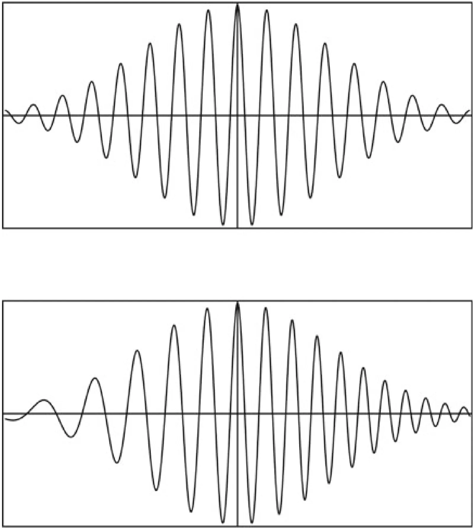
The next figure compares an unchirped pulse (top, $Γ_{i} = 0$ ) and a chirped pulse (bottom, $Γ_{i} \neq 0$ ).

Attachments/UltraFastLasers_Keller 11.webp|700

If a pulse is chirped, its instantaneous frequency is time-dependent. The total phase of the chirped Gaussian pulse is $ϕ_{total} (t) = ω_{0} t + Γ_{i} t^{2}$ . The instantaneous frequency is:

ω (t) \equiv \frac{d ϕ_{total} (t)}{d t} = ω_{0} + 2 Γ_{i} t .

This expression shows that the instantaneous frequency varies linearly with time if $Γ_{i} \neq 0$ . The FWHM pulse duration $τ_{p}$ is defined from the intensity $I (t) \sim | A (t) |^{2} = | A_{0} |^{2} \exp (- 2 Γ_{r} t^{2})$ . By setting $I (t_{p} / 2) = I (0) / 2$ :

\exp (- 2 Γ_{r} (t_{p} / 2)^{2}) = 1 / 2 ⟹ - 2 Γ_{r} (t_{p}^{2} / 4) = - \ln 2 ⟹ τ_{p}^{2} = \frac{4 \ln 2}{2 Γ_{r}} .

So, the FWHM pulse duration $τ_{p}$ is:

τ_{p} = \sqrt{\frac{2 \ln 2}{Γ_{r}}} .

A light pulse that achieves its minimal time-bandwidth product is called time-bandwidth limited, or simply transform-limited. For a given spectral amplitude distribution, a transform-limited pulse has the shortest possible pulse duration. Any additional non-linear spectral phase (chirp) results in a longer pulse duration for the same spectral width.
If the spectrum is given as a function of wavelength $λ_{0}$ (centre) and spectral width $Δ λ_{p}$ , for all pulse shapes where the fractional bandwidth is small ( $Δ f_{p} ≪ f_{0}$ , or equivalently $Δ λ_{p} ≪ λ_{0}$ ), we find the relation:

\frac{Δ f_{p}}{f_{0}} \approx \frac{Δ λ_{p}}{λ_{0}} .

2.3.2 Shortest Pulse Duration

Continuous progress in ultrashort pulse generation has led to pulse durations below $6 fs$ in the visible and near-infrared spectral range directly from lasers, and even shorter pulses via external compression techniques. Such ultrashort pulses often exhibit broad and complex spectra that do not conform to ideal pulse shapes. In such cases, specifying the pulse duration by a simple FWHM value can be insufficient or misleading. A more general pulse width measure is the root-mean-square (rms) pulse duration:

τ_{rms}^{2} = \frac{\int_{- \infty}^{\infty} (t - ⟨ t ⟩)^{2} I (t) d t}{\int_{- \infty}^{\infty} I (t) d t} = \frac{\int_{- \infty}^{\infty} (t - ⟨ t ⟩)^{2} | E (t) |^{2} d t}{\int_{- \infty}^{\infty} | E (t) |^{2} d t}

where

⟨ t ⟩ = \frac{\int_{- \infty}^{\infty} t I (t) d t}{\int_{- \infty}^{\infty} I (t) d t}

is the temporal centre of gravity. It can be shown that, for a given power spectrum $| E (ω) |^{2}$ , the shortest rms pulse duration is obtained when the spectral phase $Φ (ω)$ is flat (constant) or at most linear with frequency ( $Φ (ω) = ϕ_{0} + ϕ_{1} ω$ ). A linear spectral phase only corresponds to a constant time shift of the pulse without affecting its duration.

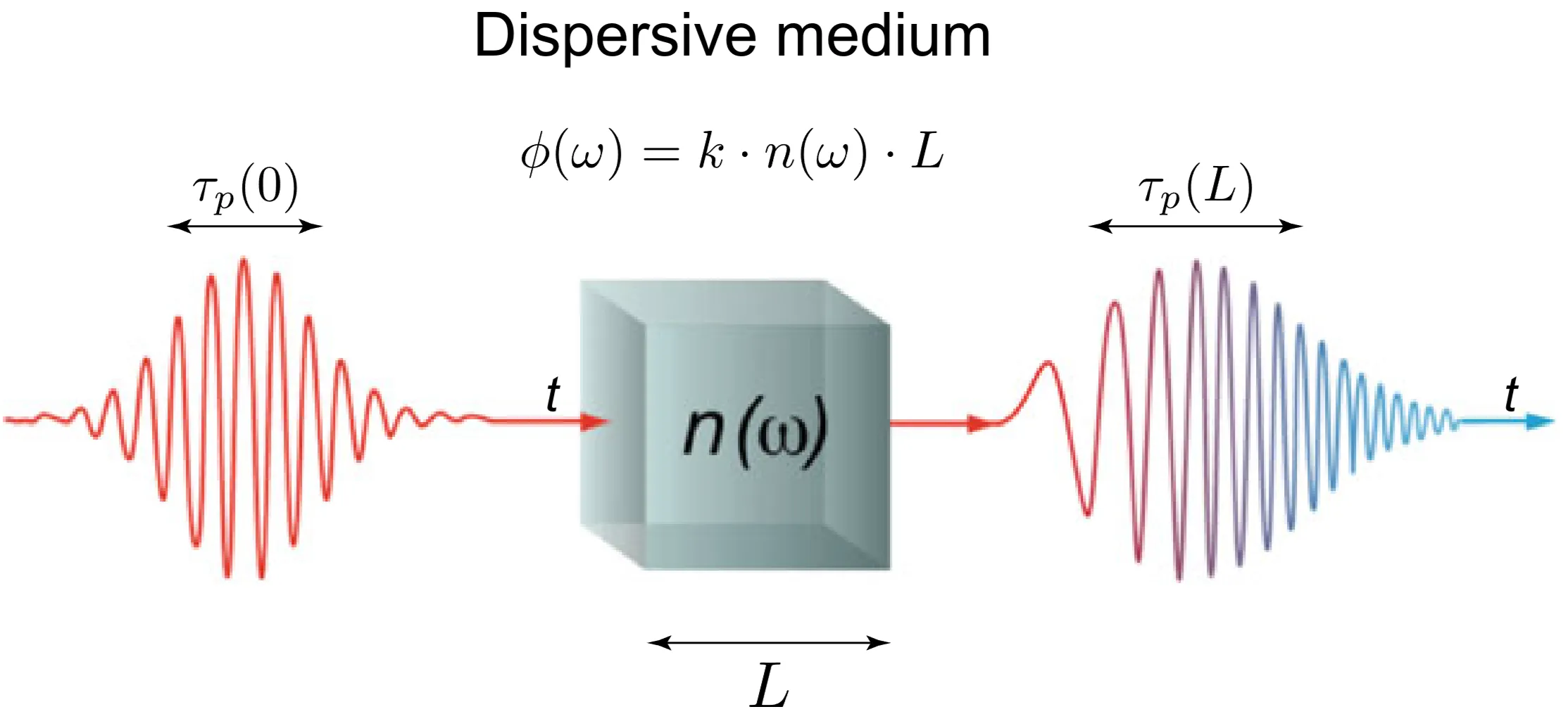
2.4 Linear pulse Propagation in a Dispersive Material

Before beginning this section, it is important to clarify that linear pulse propagation means that no intensity-dependent material properties (nonlinear optical effects like the Kerr effect) are considered. However, the refractive index $n (ω)$ of the medium can have any arbitrary (potentially highly non-linear as a function of $ω$ ) frequency dependence, leading to dispersion.

2.4.1 Slowly-Varying-Envelope Approximation

To examine the propagation of a pulse envelope $A (z, t)$ through a dispersive medium, it is useful to separate the fast optical carrier oscillation from the envelope dynamics. We write the electric field as:

E (z, t) = A (z, t) e^{i [ω_{0} t - k_{n} (ω_{0}) z]} .

The Fourier transforms $E (z, ω)$ and $A (z, Δ ω)$ (where $A (z, Δ ω)$ is the spectrum of $A (z, t)$ with respect to $t$ , and $Δ ω = ω - ω_{0}$ ) satisfy the relation:

E (z, ω_{0} + Δ ω) = A (z, Δ ω) e^{- i k_{n} (ω_{0}) z} .

Now we introduce the slowly-varying-envelope approximation (SVEA). This approximation states that the pulse envelope $A (z, t)$ changes slowly in space (over a distance $z$ ) and time (over a period $1 / ω_{0}$ ) compared to the optical carrier. Specifically for spatial variation, it assumes the envelope does not change much over a distance of one wavelength $λ_{0} / n (ω_{0})$ :

| \frac{\partial^{2} A (z, Δ ω)}{\partial z^{2}} | ≪ | 2 k_{n} (ω_{0}) \frac{\partial A (z, Δ ω)}{\partial z} | .

With this, and starting from the Helmholtz equation for $E (z, ω)$ , one can derive a simpler first-order differential equation for the evolution of the envelope's spectrum $A (z, Δ ω)$ :

\frac{\partial}{\partial z} A (z, Δ ω) + i Δ k_{n} (Δ ω) A (z, Δ ω) = 0,

where $Δ k_{n} (Δ ω) = k_{n} (ω_{0} + Δ ω) - k_{n} (ω_{0})$ . The solution to this equation is:

A (z, Δ ω) = A (0, Δ ω) e^{- i Δ k_{n} (Δ ω) z} = A (0, Δ ω) e^{- i [k_{n} (ω_{0} + Δ ω) - k_{n} (ω_{0})] z} .

This equation shows that each spectral component $A (0, Δ ω)$ of the initial envelope accumulates a phase shift $e^{- i [k_{n} (ω_{0} + Δ ω) - k_{n} (ω_{0})] z}$ as it propagates through the medium.

2.4.2 First and Second Order Dispersion

As stated before, an optical pulse is a superposition of monochromatic plane waves, where each spectral component propagates with its own phase velocity $v_{p} (ω) = ω / k_{n} (ω)$ . This frequency-dependent phase velocity (dispersion) leads to relative phase shifts between individual spectral components during propagation. Pulse broadening and distortion are primarily caused by the dispersion of the group velocity, not directly by the phase velocity dispersion.
The shorter a pulse (and thus the broader its spectrum $Δ ω$ ), the more pronounced the effects of dispersion become. Assuming the pulse bandwidth $Δ ω$ is small compared to the carrier frequency $ω_{0}$ ( $Δ ω ≪ ω_{0}$ ), we may expand the wave number $k_{n} (ω)$ in a Taylor series around $ω_{0}$ :

k_{n} (ω) \approx k_{n} (ω_{0}) + k_{n}^{'} (ω_{0}) (ω - ω_{0}) + \frac{1}{2} k_{n}^{''} (ω_{0}) (ω - ω_{0})^{2} + \dots,

where $Δ ω = ω - ω_{0}$ .
$k_{n}^{'} (ω_{0}) = {\frac{d k_{n}}{d ω} |}_{ω_{0}}$ is the first-order dispersion coefficient (inverse group velocity).
$k_{n}^{''} (ω_{0}) = {\frac{d^{2} k_{n}}{d ω^{2}} |}_{ω_{0}}$ is the second-order dispersion coefficient, often called Group Velocity Dispersion (GVD) parameter.
This expansion is typically valid in the optical region even for ultrashort pulses of several femtoseconds.

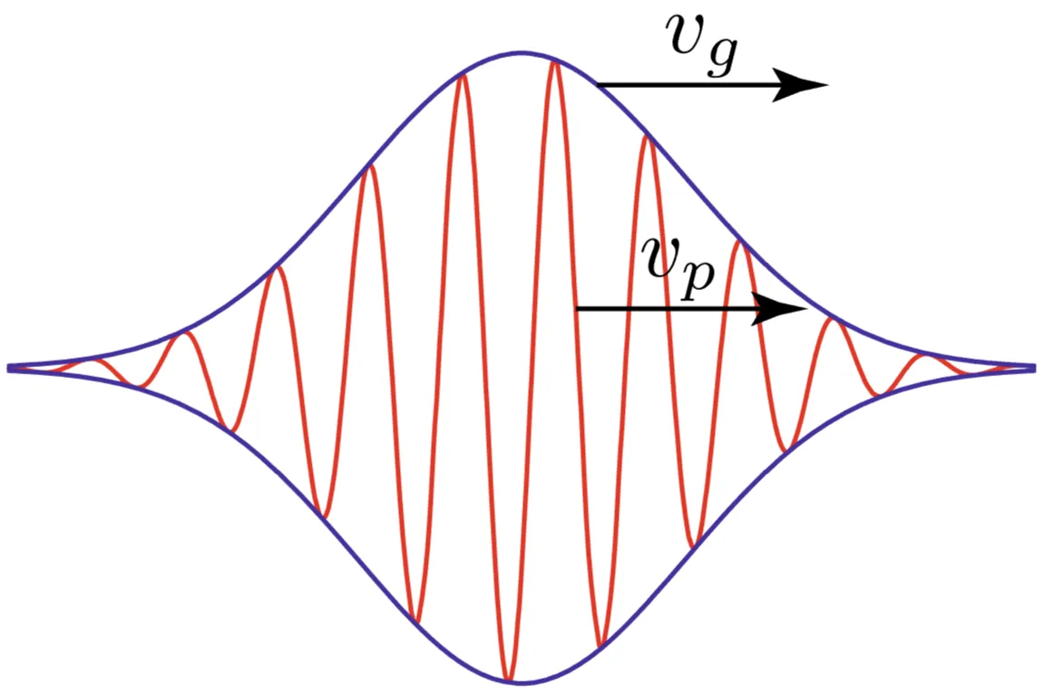
2.4.3 Phase Velocity and Group Velocity

For a Gaussian pulse, linear pulse propagation including up to second-order dispersion can often be solved analytically. The phase velocity is defined as:

v_{p} (ω_{0}) = \frac{ω_{0}}{k_{n} (ω_{0})} = \frac{c}{n (ω_{0})} .

The group velocity $v_{g}$ is defined as:

v_{g} (ω_{0}) = {({\frac{d k_{n}}{d ω} |}_{ω_{0}})}^{- 1} = \frac{1}{k_{n}^{'} (ω_{0})} .

The phase velocity describes the propagation velocity of the carrier wave (surfaces of constant phase). The group velocity corresponds to the propagation velocity of the peak of the pulse envelope (under certain approximations).

Attachments/UltraFastLasers_Keller 12.webp|700

In vacuum, $n (ω) = 1$ , so $k_{n} (ω) = ω / c$ , $k_{n}^{'} (ω) = 1 / c$ , $k_{n}^{″} (ω) = 0$ . Thus $v_{p} = c$ and $v_{g} = c$ .
The first-order dispersion $k_{n}^{'}$ determines the overall temporal shift of the pulse, quantified by the group delay $T_{g}$ after propagating a distance $z$ :

T_{g} (z) = k_{n}^{'} z = \frac{z}{v_{g}} .

2.4.4 Pulse Broadening

A pulse is temporally broadened (or compressed, depending on initial chirp and dispersion sign) by propagation through a dispersive medium. Remember that a linear system cannot spectrally broaden or narrow the pulse; $| E (z, ω) |^{2}$ remains unchanged if the medium is lossless.

Attachments/UltraFastLasers_Keller 13.webp|700

This temporal reshaping can be seen by considering the FWHM pulse duration of an initially unchirped Gaussian pulse with initial duration $τ_{p} (0)$ and complex parameter $Γ (0) = Γ_{r} (0)$ . After propagating a distance $L_{d}$ , the pulse acquires chirp and its new complex parameter is $Γ (L_{d})$ . The duration becomes:

τ_{p} (L_{d}) = \sqrt{\frac{2 \ln 2}{Re [Γ (L_{d})]}} .

The first-order dispersion term ( $k_{n}^{'}$ ) only causes a temporal shift (group delay) and does not contribute to pulse broadening. Only second-order dispersion ( $k_{n}^{″}$ , GVD) and higher-order dispersion terms cause changes in pulse duration and shape for an initially unchirped pulse.
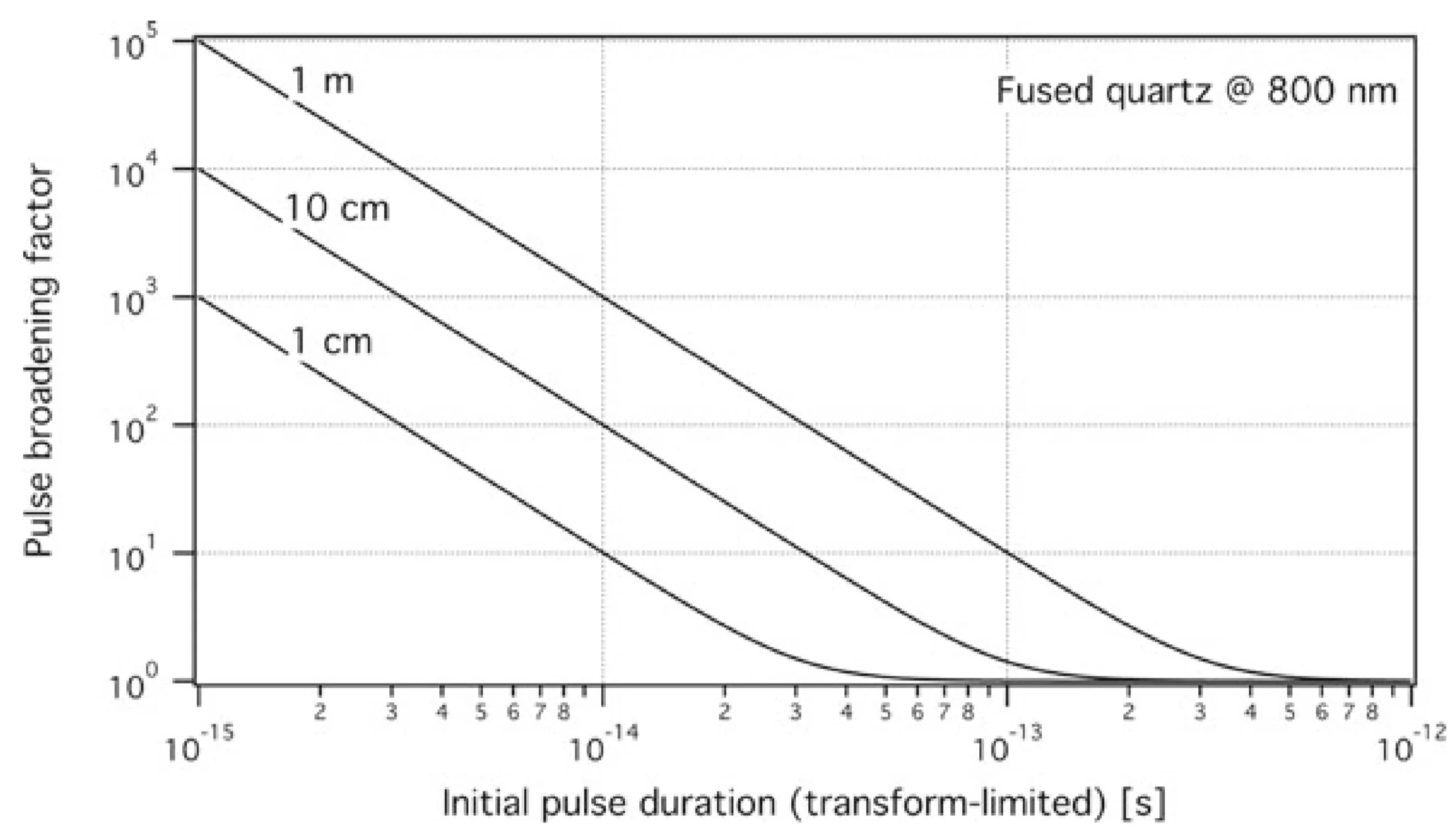
For an initially transform-limited Gaussian pulse of duration $τ_{p} (0)$ , after propagating a distance $L_{d}$ in a medium with GVD $k_{n}^{″}$ , the duration becomes:

\frac{τ_{p} (L_{d})}{τ_{p} (0)} = \sqrt{1 + {(\frac{k_{n}^{''} L_{d} (4 \ln 2)}{τ_{p}^{2} (0)})}^{2}} = \sqrt{1 + {(\frac{GDD}{τ_{p}^{2} (0) / (2 \ln 2)} \frac{2}{τ_{p} (0)})}^{2}} .

Here, GDD (Group Delay Dispersion) is $\frac{d^{2} ϕ}{d ω^{2}} = k_{n}^{″} L_{d}$ . The formula shows that the shorter the original pulse $τ_{p} (0)$ (meaning larger spectral bandwidth), the more it is stretched in time by a given amount of GDD. The next figure shows the pulse broadening factor for Gaussian pulses of different initial durations passing through a $1 cm$ thick fused silica lens.

Attachments/UltraFastLasers_Keller 14.webp|700

Strong Pulse Broadening Approximation
The case of strong pulse broadening occurs when the second term under the square root is much larger than 1, which means the accumulated GDD is large compared to $τ_{p}^{2} (0) / (4 \ln 2)$ . This is often stated as when the propagation distance $L_{d}$ is much greater than the "dispersion length" $L_{D} = τ_{p}^{2} (0) / (4 \ln 2 | k_{n}^{″} |)$ . Equivalently:

| GDD | = | k_{n}^{''} | L_{d} ≫ \frac{τ_{p}^{2} (0)}{4 \ln 2} .

In this limit, assuming an unchirped initial Gaussian pulse of spectral FWHM $Δ ω_{p} = 4 \ln 2 / τ_{p} (0)$ :

τ_{p} (L_{d}) \approx \frac{| k_{n}^{''} | L_{d} (4 \ln 2)}{τ_{p} (0)} = | GDD | \frac{4 \ln 2}{τ_{p} (0)} = | GDD | Δ ω_{p} .

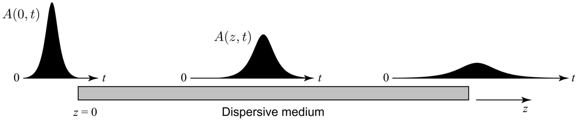
The effect of an unchirped pulse passing through a dispersive medium (with, say, positive $k_{n}^{″}$ ) is schematically shown here:

Attachments/UltraFastLasers_Keller 15.webp|700

The pulse becomes longer and acquires a linear chirp. For positive $k_{n}^{″}$ (normal dispersion in typical glass for visible light), higher frequencies (blue) travel slower than lower frequencies (red). An initially unchirped pulse develops a positive chirp (red leading blue).

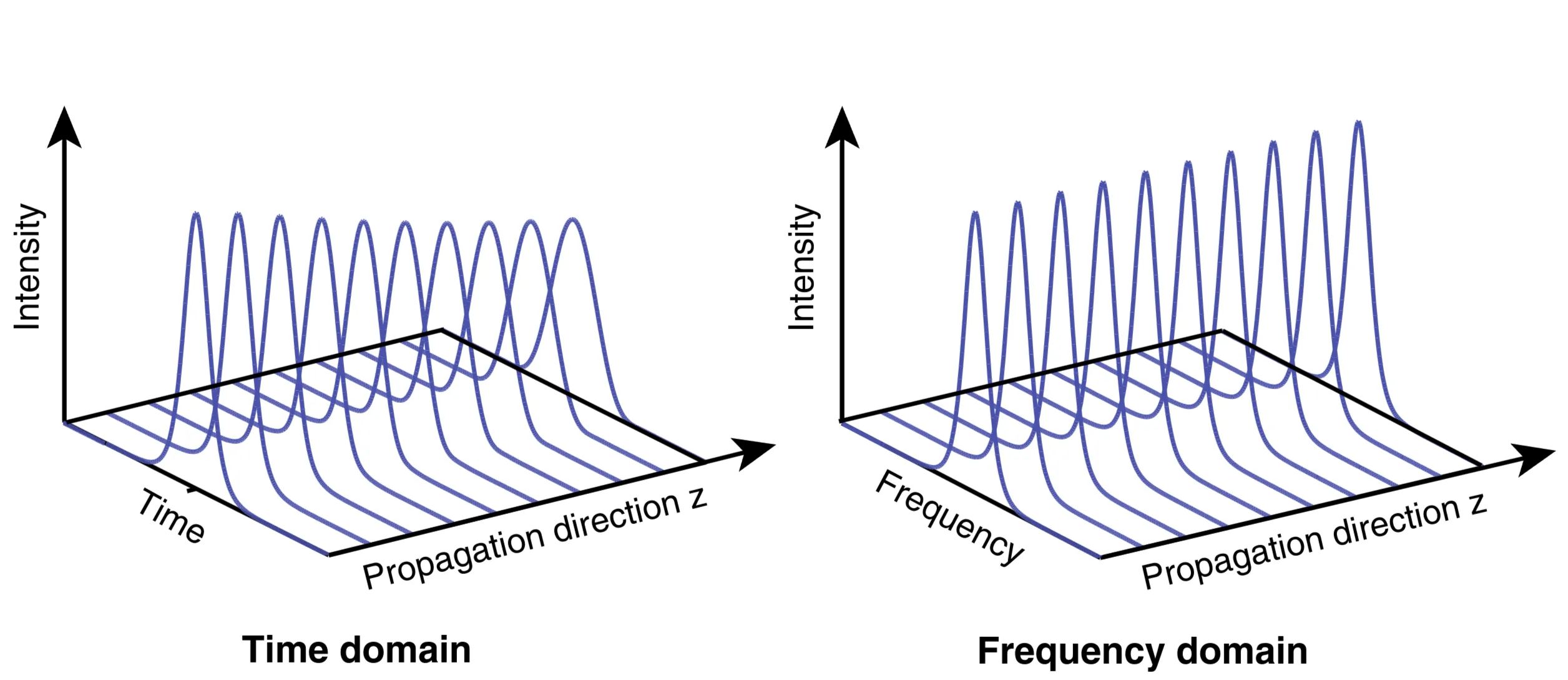
Normal dispersion (e.g. k_{n}^{″} > 0) : v_{g} (ω_{blue}) < v_{g} (ω_{red}) .

The broadened pulse is chirped by the dispersion. However, as mentioned, the pulse power spectrum $| E (z, ω) |^{2}$ does not change during linear propagation in a lossless medium:

Attachments/UltraFastLasers_Keller 16.webp|700

Linear dispersive pulse broadening (for initially unchirped pulses) arises from second-order and higher-order dispersion. It is therefore the frequency dependence of the group velocity (related to $k_{n}^{″}$ ) that is primarily responsible for this broadening, not the frequency dependence of the phase velocity itself.

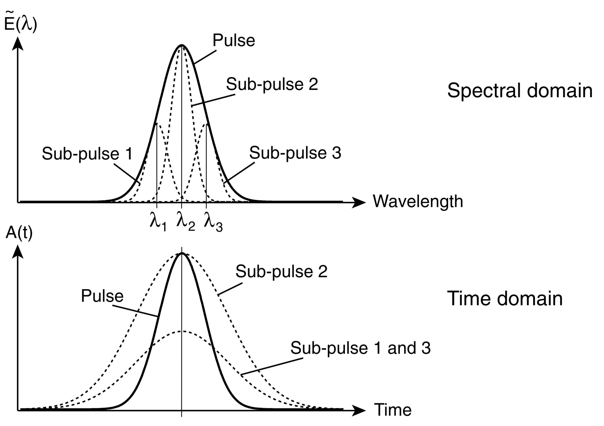
This can be depicted as in the following figure. Consider that a short pulse can be thought of as a superposition of many longer sub-pulses, each with a slightly different centre wavelength/frequency. The superposition results in a short overall pulse because the electric fields in the wings of the sub-pulses interfere destructively:

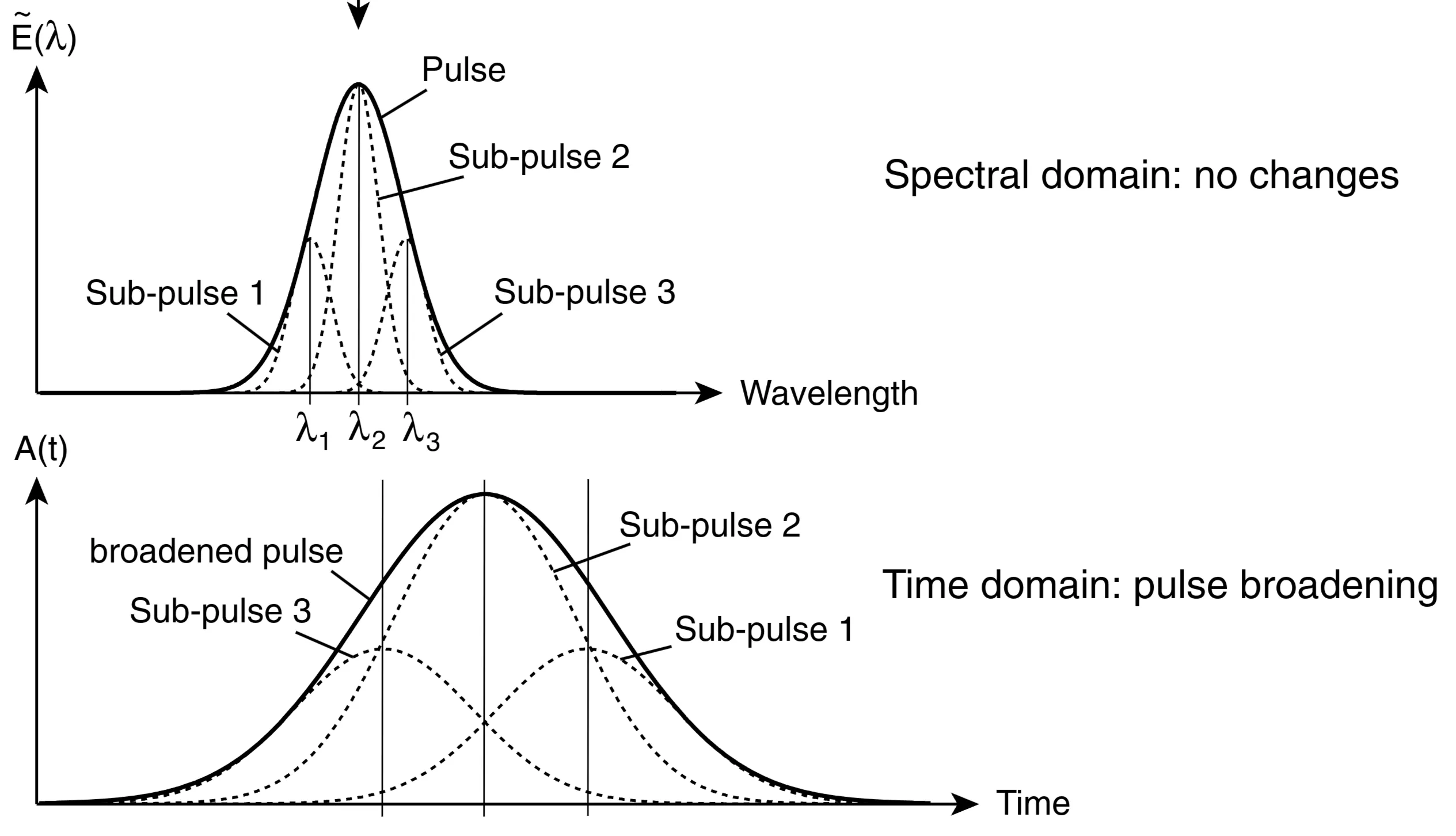
Attachments/UltraFastLasers_Keller 17.webp|700

Now observe what happens when this collection of sub-pulses passes through a dispersive medium:

Attachments/UltraFastLasers_Keller 18.webp|700

Note that, in this conceptual picture, the individual sub-pulses (if they were narrow enough in spectrum not to experience significant GVD themselves) do not broaden significantly. Rather, the broadening of the resultant overall pulse comes from the fact that these sub-pulses, with their slightly different centre frequencies, travel at different group velocities through the dispersive medium. This differential group delay causes them to spread out in time, leading to broadening of the total pulse.

It is useful to know dispersion parameters as a function of both frequency $ω$ and wavelength $λ$ (where $n^{'} = d n / d λ$ , $n^{″} = d^{2} n / d λ^{2}$ etc.):

Dispersion parameter	Definition	Calculation from $n (λ)$
Phase velocity $v_{p}$	$ω / k_{n} (ω)$	$c / n (λ)$
Group velocity $v_{g}$	$(d k_{n} / d ω)^{- 1}$	$\frac{c}{n (λ) - λ n^{'} (λ)}$
Group delay $T_{g}$ (per unit length $L_{d}$ )	$k_{n}^{'} = d k_{n} / d ω = 1 / v_{g}$	$\frac{1}{c} (n (λ) - λ n^{'} (λ))$
GDD (Group Delay Dispersion, total over $L_{d}$ )	$k_{n}^{″} L_{d} = d^{2} (k_{n} L_{d}) / d ω^{2}$	$\frac{λ^{3} L_{d}}{2 π c^{2}} n^{″} (λ)$ [units: ${fs}^{2}$ ]
Dispersion parameter $D_{λ}$ (GDD per unit length and $Δ λ$ )	$\frac{1}{L_{d}} \frac{d T_{g}}{d λ} = - \frac{2 π c}{λ^{2}} k_{n}^{″}$	$- \frac{λ}{c} n^{″} (λ)$ [units: $ps/(nm km)$ or $fs/(nm cm)$ ]
TOD (Third Order Dispersion, total over $L_{d}$ )	$k_{n}^{‴} L_{d} = d^{3} (k_{n} L_{d}) / d ω^{3}$	$- \frac{λ^{4} L_{d}}{(2 π c)^{2} c} (3 n^{″} (λ) + λ n^{‴} (λ))$ [units: ${fs}^{3}$ ]

Different units and definitions for GVD/GDD are used depending on the application.

2.4.5 Can a Pulse Propagate Faster than the Speed of Light in Vacuum?

The proof is skipped, but the group velocity $v_{g}$ can, under certain conditions (such as near an absorption resonance in a region of anomalous dispersion), be greater than the speed of light in vacuum $c$ , or even negative. However, this is not a contradiction with the theory of relativity. No information or energy can be transmitted with superluminal velocity.
The argument that because a Gaussian pulse is analytical, its future is determined by its past, and thus its peak propagation does not represent signal velocity, is one perspective. More rigorously, the front velocity of any signal (the speed of its very first non-zero disturbance) cannot exceed $c$ .
It is useful to define the group index $n_{g}$ :

n_{g} (ω) = n (ω) + ω \frac{d n (ω)}{d ω} = n (λ) - λ \frac{d n (λ)}{d λ},

such that $v_{g} (ω) = c / n_{g} (ω)$ .

2.4.6 Higher Order Dispersion

While pulses with durations of $10 - 30 fs$ can be generated relatively straightforwardly, increasing difficulties arise for generating and propagating even shorter durations. For such extremely short pulses (few-cycle or single-cycle), higher-order dispersion terms beyond GVD (like third-order dispersion, TOD, related to $k_{n}^{‴}$ ) become more important. To characterise their relative importance, dispersion lengths can be introduced:

L_{D} = \frac{τ_{0}^{2}}{| k_{n}^{″} |}, L_{D}^{'} = \frac{τ_{0}^{3}}{| k_{n}^{‴} |},

where $τ_{0}$ is a characteristic initial pulse duration (related to, but not necessarily equal to, $τ_{p} (0)$ FWHM). Third-order dispersion significantly affects pulse propagation if $L_{D}^{'}$ becomes comparable to or smaller than $L_{D}$ , or comparable to the actual propagation length $z$ . Similar arguments apply for even higher orders of dispersion.
The formula for pulse broadening for $z ≫ L_{D}$ that includes TOD,

\frac{τ_{p} (z)}{τ_{p} (0)} \approx z \sqrt{1 + \frac{1}{L_{D}^{2}} + \frac{1}{4 L_{D}^{' 2}}} .