Jump back to chapter selection.

Table of Contents

9.1 Many-Body Wave Functions and Particle Statistics
9.2 Independent, Indistinguishable Particles
9.3 Second Quantisation Formalism
9.4 Observables in Second Quantisation
9.5 Equation of Motion
9.6 Correlation Functions
9.7 Selected Applications

9 Identical Quantum Particles - Formalism of Second Quantisation

This chapter gives an introduction to the formalism of second quantisation, which is a convenient technical tool for discussing many-body quantum systems. It is indispensable in quantum field theory as well as in solid state physics. We distinguish between fermions (half-integer spins) and bosons (integer spins), which behave quite differently, as we have seen in the previous chapter. This behaviour is implemented in their many-body wave functions. While in the previous chapter we could circumvent dealing with this aspect as we considered independent, indistinguishable quantum particles, it is unavoidable to implement a more careful analysis once interactions between the particles appear.

9.1 Many-Body Wave Functions and Particle Statistics

The Hamiltonian describing the dynamics of a system of many identical quantum particles must be invariant under exchange (permutation) of particle degrees of freedom (coordinate, momentum, spin, and so forth). The identical quantum particles are indistinguishable, since in quantum mechanics it is impossible to follow the trajectories of particles under general conditions, unlike in classical mechanics. Permutations play indeed an important role in characterising quantum particles. We introduce the many-body wave function of $N$ particles,

\begin{array}{r} ψ (r_{1}, s_{1}; r_{2}, s_{2}; \dots; r_{N}, s_{N}) \end{array}

where each particle is labeled by the coordinate $r$ and spin $s$ . In the following we will use for this the shorthand notation $ψ (1, \dots, N)$ . Analogously we define many-body operators,

\begin{array}{r} \hat{A} (1, \dots, N) = A ({\hat{r}}_{1}, {\hat{p}}_{1}, {\hat{S}}_{1}; \dots; {\hat{r}}_{N}, {\hat{p}}_{N}, {\hat{S}}_{N}) \end{array}

with ${\hat{r}}_{j}, {\hat{p}}_{j}$ and ${\hat{S}}_{j}$ being the operators for position, momentum and spin of particle $j$ . Note that the Hamiltonian $H$ belongs to these operators as well.
We introduce the transposition (exchange) operator ${\hat{P}}_{i j}$ , which is an element of the permutation group of $N$ elements and exchanges particles $i$ and $j$ ( $1 \leq i, j \leq N$ ),

\begin{array}{r} \begin{aligned} {\hat{P}}_{i j} ψ (1, \dots, i, \dots, j, \dots, N) = ψ (1, \dots, j, \dots, i, \dots, N) \\ {\hat{P}}_{i j} \hat{A} (1, \dots, i, \dots, j, \dots, N) = \hat{A} (1, \dots, j, \dots, i, \dots, N) \end{aligned} \end{array}

Note that ${({\hat{P}}_{i j})}^{- 1} = {\hat{P}}_{i j}$ . As the Hamiltonian is invariant under particle exchange, it commutes with ${\hat{P}}_{i j}$ ,

\begin{array}{r} [H, {\hat{P}}_{i j}] = 0 \end{array}

and, consequently, any combination of several transpositions, meaning all elements of the permutation group $S_{N}$ , commutes with $H$ . Hence, eigenstates of $H$ have the property

\begin{array}{r} H | ψ ⟩ = E | ψ ⟩ \Rightarrow H {\hat{P}}_{i j} | ψ ⟩ = {\hat{P}}_{i j} H | ψ ⟩ = E {\hat{P}}_{i j} | ψ ⟩, \end{array}

where we define the wave function as

\begin{array}{r} ψ (1, \dots, N) = ⟨ 1, \dots, N ∣ ψ ⟩ . \end{array}

We distinguish now between fermions and bosons through their behaviour under transpositions ${\hat{P}}_{i j}$ ,

\begin{array}{r} ψ (1, \dots, i, \dots, j, \dots, N) = {\begin{cases} + ψ (1, \dots, j, \dots, i, \dots, N) & bosons \\ - ψ (1, \dots, j, \dots, i, \dots, N) & fermions \end{cases} \end{array}

This means that bosonic wave functions are completely symmetric under exchange of particles, while fermionic wave functions are completely antisymmetric. Note that this property is valid also for composite particles. Any particle composed of an even number of constituent fermions would be a boson; for instance, $^{4} He$ (2 protons + 2 neutrons + 2 electrons = 6 fermions). Exchanging two such composite particles leaves the sign of the wave function unchanged. In the same way a particle with an odd number of constituent fermions is a fermion; for instance, $^{3}$ He (2 protons + 1 neutron + 2 electrons = 5 fermions). Note that the antisymmetric wave functions prevent two fermions from having the same quantum numbers. If $(r_{i}, s_{i})$ and $(r_{j}, s_{j})$ are identical, then we find

\begin{array}{r} ψ (1, \dots, i, \dots, i, \dots, N) = - ψ (1, \dots, i, \dots, i, \dots, N) = 0 \end{array}

which implies the Pauli exclusion principle.

9.2 Independent, Indistinguishable Particles

We consider $N$ identical particles in a potential $V$ which are not interacting with each other. The Hamiltonian is then given by

\begin{array}{r} H = \sum_{i = 1}^{N} H_{i} with H_{i} = \frac{{\hat{p}}_{i}^{2}}{2 m} + V ({\hat{r}}_{i}) . \end{array}

The states of each particle, described by single-particle wave functions $ψ_{ν}$ , form a basis for the single-particle Hilbert space, and we can find the stationary states

\begin{array}{r} H_{i} ψ_{ν} (r_{i}, s_{i}) = ϵ_{ν} ψ_{ν} (r_{i}, s_{i}) . \end{array}

These single-particle wave functions are normalised, meaning

\begin{array}{r} \sum_{s} \int d^{3} r {| ψ_{ν} (r, s) |}^{2} = 1 \end{array}

We may now construct a many-body wave function as a product wave function with the corresponding exchange property.
For bosons, we write

\begin{array}{r} ⟨ r_{1}, s_{1}; \dots, r_{N}, s_{N} ∣ Ψ_{B} ⟩ = Ψ_{B} (1, \dots, N) = N_{B} \sum_{\hat{P} \in S_{N}} \hat{P} (ψ_{ν_{1}} (1) \dots ψ_{ν_{N}} (N)) \end{array}

and for fermions

\begin{array}{r} ⟨ r_{1}, s_{1}; \dots, r_{N}, s_{N} ∣ Ψ_{F} ⟩ = Ψ_{F} (1, \dots, N) = N_{F} \sum_{\hat{P} \in S_{N}} sgn (\hat{P}) \hat{P} (ψ_{ν_{1}} (1) \dots ψ_{ν_{N}} (N)) \end{array}

where $\hat{P}$ permutes the particle labels $(1, \dots, N)$ in the product of single-particle wave functions $ψ_{ν_{i}} (j)$ , $sgn (\hat{P})$ is the sign of the permutation $\hat{P}$ which is $+ 1 (- 1)$ if $\hat{P}$ is composed of an even (odd) number of transpositions, and $N_{B}, N_{F}$ are normalisation constants. Interestingly the fermionic wave function can be represented as a determinant, the so-called Slater determinant,

\begin{array}{r} Ψ_{F} (1, \dots, N) = \frac{1}{\sqrt{N!}} Det [\begin{array}{ccc} ψ_{ν_{1}} (1) & \dots & ψ_{ν_{1}} (N) \\ ⋮ & ⋮ \\ ψ_{ν_{N}} (1) & \dots & ψ_{ν_{N}} (N) \end{array}] \end{array}

Obviously the determinant vanishes if two rows (identical states $ν_{i} = ν_{j}$ ) or columns (identical particles $i = j$ ) are identical, enforcing the Pauli principle. These wave functions (as constructed by the sums over permutations without explicit $N$ ) are not yet normalised. Their norms are:

\begin{array}{r} \begin{aligned} ⟨ Ψ_{B}^{unnorm} ∣ Ψ_{B}^{unnorm} ⟩ = N! n_{ν_{1}}! \dots n_{ν_{k}}! (sum over distinct states k), \\ ⟨ Ψ_{F}^{unnorm} ∣ Ψ_{F}^{unnorm} ⟩ = N!, \end{aligned} \end{array}

where $n_{ν_{j}}$ denotes the number of particles in the single-particle state labeled by $ν_{j}$ . For fermions, $n_{ν_{j}}$ can only be $0$ or $1$ .

9.3 Second Quantisation Formalism

It is in principle possible to investigate many-body states using many-body wave functions. However, we will introduce here a formalism that is in many respects much more convenient and efficient. It is based on the operators which "create" or "annihilate" particles and act on states in the Fock space $F$ , which is an extended space of states combining Hilbert spaces $Q_{n}$ for different particle numbers $n$ ,

\begin{array}{r} F = ⨁_{n = 0}^{\infty} Q_{n} . \end{array}

Note that the name "second quantisation" does not imply a new quantum mechanics.
We can express a many-body state of independent particles in the occupation number representation,

\begin{array}{r} | n_{ν_{1}}, n_{ν_{2}}, \dots ⟩ \end{array}

which is a state in $F$ whose particle number is given by $N = n_{ν_{1}} + n_{ν_{2}} + \dots$ .

9.3.1 Creation- and Annihilation Operators

We define operators ${\hat{a}}_{ν}$ and ${\hat{a}}_{ν}^{†}$ which connect Hilbert spaces of different particle number,

\begin{array}{r} {\hat{a}}_{ν} : Q_{n} \to Q_{n - 1} and {\hat{a}}_{ν}^{†} : Q_{n} \to Q_{n + 1} . \end{array}

The first is called an annihilation operator and the second a creation operator; their action is best understood in the occupation number representation.

Bosons: Let us first consider bosons which, for simplicity, do not possess spin. The two operators have the following property,

\begin{array}{r} \begin{aligned} {\hat{a}}_{ν} | n_{ν_{1}}, n_{ν_{2}}, \dots, n_{ν}, \dots ⟩ = \sqrt{n_{ν}} | n_{ν_{1}}, n_{ν_{2}}, \dots, n_{ν} - 1, \dots ⟩, \\ {\hat{a}}_{ν}^{†} | n_{ν_{1}}, n_{ν_{2}}, \dots, n_{ν}, \dots ⟩ = \sqrt{n_{ν} + 1} | n_{ν_{1}}, n_{ν_{2}}, \dots, n_{ν} + 1, \dots ⟩, \end{aligned} \end{array}

and their adjoint actions are

\begin{array}{r} \begin{aligned} ⟨ n_{ν_{1}}, n_{ν_{2}}, \dots, n_{ν}, \dots | {\hat{a}}_{ν}^{†} = \sqrt{n_{ν}} ⟨ n_{ν_{1}}, n_{ν_{2}}, \dots, n_{ν} - 1, \dots |, \\ ⟨ n_{ν_{1}}, n_{ν_{2}}, \dots, n_{ν}, \dots | {\hat{a}}_{ν} = \sqrt{n_{ν} + 1} ⟨ n_{ν_{1}}, n_{ν_{2}}, \dots, n_{ν} + 1, \dots | . \end{aligned} \end{array}

It is obvious that

\begin{array}{r} {\hat{a}}_{ν} | \dots, n_{ν} = 0, \dots ⟩ = 0 and (from the above definition for bras) ⟨ \dots, n_{ν} = 0, \dots | {\hat{a}}_{ν}^{†} = 0 \end{array}

The operators satisfy the following commutation relations,

\begin{array}{r} [{\hat{a}}_{ν}, {\hat{a}}_{ν^{'}}^{†}] = δ_{ν ν^{'}} and [{\hat{a}}_{ν}, {\hat{a}}_{ν^{'}}] = [{\hat{a}}_{ν}^{†}, {\hat{a}}_{ν^{'}}^{†}] = 0 \end{array}

Note that these relations correspond to those of the lowering and raising operators of a harmonic oscillator. Indeed we have seen previously that the excitation spectrum of a harmonic oscillator obeys bosonic statistics.
The creation operators can also be used to construct a state from the vacuum, denoted as $| 0 ⟩$ , where there are no particles, such that ${\hat{a}}_{ν} | 0 ⟩ = 0$ for all $ν$ . A general state in occupation number representation can be written as,

\begin{array}{r} | n_{ν_{1}}, n_{ν_{2}}, \dots, n_{ν}, \dots ⟩ = \frac{{({\hat{a}}_{ν_{1}}^{†})}^{n_{ν_{1}}}}{\sqrt{n_{ν_{1}}!}} \frac{{({\hat{a}}_{ν_{2}}^{†})}^{n_{ν_{2}}}}{\sqrt{n_{ν_{2}}!}} \dots \frac{{({\hat{a}}_{ν_{k}}^{†})}^{n_{ν_{k}}}}{\sqrt{n_{ν_{k}}!}} \dots | 0 ⟩ \end{array}

The number operator is defined as

\begin{array}{r} {\hat{n}}_{ν} = {\hat{a}}_{ν}^{†} {\hat{a}}_{ν} with {\hat{n}}_{ν} | \dots, n_{ν}, \dots ⟩ = n_{ν} | \dots, n_{ν}, \dots ⟩ \end{array}

and the total number of particles is obtained through the operator

\begin{array}{r} \hat{N} = \sum_{i} {\hat{n}}_{ν_{i}} \end{array}

Knowing the spectrum of the Hamiltonian of independent particles, we may express the Hamiltonian as

\begin{array}{r} H = \sum_{ν} ϵ_{ν} {\hat{a}}_{ν}^{†} {\hat{a}}_{ν} = \sum_{ν} ϵ_{ν} {\hat{n}}_{ν} \end{array}

Fermions: Now we turn to fermions with spin $1 / 2$ (or any half-integer spin). Again the single-particle state will be labelled by $ν$ including the spin index for $↑$ and $↓$ . Analogously to the case of bosons, we introduce operators ${\hat{c}}_{ν}^{†}$ and ${\hat{c}}_{ν}$ (using $c$ for fermions to distinguish from bosonic $a$ ) which obey anti-commutation rules,

\begin{array}{r} {{\hat{c}}_{ν}, {\hat{c}}_{ν^{'}}^{†}} = δ_{ν ν^{'}} and {{\hat{c}}_{ν}, {\hat{c}}_{ν^{'}}} = {{\hat{c}}_{ν}^{†}, {\hat{c}}_{ν^{'}}^{†}} = 0 \end{array}

where ${\hat{A}, \hat{B}} = \hat{A} \hat{B} + \hat{B} \hat{A}$ . In particular this implies that

\begin{array}{r} {\hat{c}}_{ν}^{†} {\hat{c}}_{ν}^{†} = 0 and {\hat{c}}_{ν} {\hat{c}}_{ν} = 0 \end{array}

such that $n_{ν} = 0, 1$ , meaning each single-particle state labelled by $ν$ can be occupied by at most one particle, because

\begin{array}{r} {\hat{c}}_{ν}^{†} | \dots, n_{ν} = 1, \dots ⟩ = {\hat{c}}_{ν}^{†} {\hat{c}}_{ν}^{†} | \dots, n_{ν} = 0, \dots ⟩ = 0 \end{array}

A general state may be written as (assuming a standard ordering for $ν_{i}$ , for instance, increasing index)

\begin{array}{r} | n_{ν_{1}}, n_{ν_{2}}, \dots ⟩ = {({\hat{c}}_{ν_{k}}^{†})}^{n_{ν_{k}}} \dots {({\hat{c}}_{ν_{2}}^{†})}^{n_{ν_{2}}} {({\hat{c}}_{ν_{1}}^{†})}^{n_{ν_{1}}} | 0 ⟩ \end{array}

which restricts $n_{ν}$ to 0 or 1. The order of the creation operators plays an important role as the exchange of two operators yields a minus sign. We consider an example here, with a chosen ordering $ν_{1} < ν_{2} < ν_{3} < ν_{4}$ :

\begin{array}{r} | 1_{1}, 1_{2}, 1_{3}, 1_{4} ⟩ = {\hat{c}}_{4}^{†} {\hat{c}}_{3}^{†} {\hat{c}}_{2}^{†} {\hat{c}}_{1}^{†} | 0 ⟩ \end{array}

Removing now one particle yields

\begin{array}{r} \begin{aligned} {\hat{c}}_{2} | 1_{1}, 1_{2}, 1_{3}, 1_{4} ⟩ & = {\hat{c}}_{2} [{\hat{c}}_{4}^{†} {\hat{c}}_{3}^{†} {\hat{c}}_{2}^{†} {\hat{c}}_{1}^{†}] | 0 ⟩ \\ = (- 1)^{2} {\hat{c}}_{4}^{†} {\hat{c}}_{3}^{†} {\hat{c}}_{2} {\hat{c}}_{2}^{†} {\hat{c}}_{1}^{†} | 0 ⟩ (moving {\hat{c}}_{2} past {\hat{c}}_{4}^{†}, {\hat{c}}_{3}^{†}) \\ = {\hat{c}}_{4}^{†} {\hat{c}}_{3}^{†} (1 - {\hat{c}}_{2}^{†} {\hat{c}}_{2}) {\hat{c}}_{1}^{†} | 0 ⟩ \\ = {\hat{c}}_{4}^{†} {\hat{c}}_{3}^{†} {\hat{c}}_{1}^{†} | 0 ⟩ = | 1_{1}, 0_{2}, 1_{3}, 1_{4} ⟩ \end{aligned} \end{array}

and now analogously

\begin{array}{r} \begin{aligned} {\hat{c}}_{3} | 1_{1}, 1_{2}, 1_{3}, 1_{4} ⟩ & = {\hat{c}}_{3} [{\hat{c}}_{4}^{†} {\hat{c}}_{3}^{†} {\hat{c}}_{2}^{†} {\hat{c}}_{1}^{†}] | 0 ⟩ \\ = (- 1)^{1} {\hat{c}}_{4}^{†} {\hat{c}}_{3} {\hat{c}}_{3}^{†} {\hat{c}}_{2}^{†} {\hat{c}}_{1}^{†} | 0 ⟩ (moving {\hat{c}}_{3} past {\hat{c}}_{4}^{†}) \\ = - {\hat{c}}_{4}^{†} (1 - {\hat{c}}_{3}^{†} {\hat{c}}_{3}) {\hat{c}}_{2}^{†} {\hat{c}}_{1}^{†} | 0 ⟩ \\ = - {\hat{c}}_{4}^{†} {\hat{c}}_{2}^{†} {\hat{c}}_{1}^{†} | 0 ⟩ = - | 1_{1}, 1_{2}, 0_{3}, 1_{4} ⟩ . \end{aligned} \end{array}

Obviously, the order of the operators is important and should not be ignored when dealing with fermions. A consistent phase convention (for instance, Jordan-Wigner string) is required for general operations.

9.3.2 Field Operators

We consider now independent free particles whose states are characterised by momentum $p = ℏ k$ and spin $s$ with an energy $ϵ_{k} = ℏ^{2} k^{2} / 2 m$ . The wave functions have a plane wave form,

\begin{array}{r} ψ_{k s} (r) = \frac{1}{\sqrt{V}} e^{i k \cdot r} χ_{s} with k = \frac{2 π}{L} (n_{x}, n_{y}, n_{z}) \end{array}

where we used periodic boundary conditions in a cube of edge length $L$ (volume $V = L^{3}$ ), and $χ_{s}$ is the spin part. On this basis we write field operators (using $\hat{c}$ for fermions, $\hat{a}$ for bosons generically or when context is clear)

\begin{array}{r} {\hat{Ψ}}_{s} (r) = \frac{1}{\sqrt{V}} \sum_{k} e^{i k \cdot r} {\hat{c}}_{k s} and {\hat{Ψ}}_{s}^{†} (r) = \frac{1}{\sqrt{V}} \sum_{k} e^{- i k \cdot r} {\hat{c}}_{k s}^{†} \end{array}

and the inverse,

\begin{array}{r} {\hat{c}}_{k s}^{†} = \int d^{3} r \frac{e^{i k \cdot r}}{\sqrt{V}} {\hat{Ψ}}_{s}^{†} (r) and {\hat{c}}_{k s} = \int d^{3} r \frac{e^{- i k \cdot r}}{\sqrt{V}} {\hat{Ψ}}_{s} (r) \end{array}

Also these operators ${\hat{Ψ}}_{s} (r)$ and ${\hat{Ψ}}_{s}^{†} (r)$ act as annihilation or creation operators, respectively, in the sense,

\begin{array}{r} {\hat{Ψ}}_{s}^{†} (r) | 0 ⟩ = | r, s ⟩ and ϕ_{s} (r) = ⟨ r, s ∣ ϕ ⟩ = ⟨ 0 | {\hat{Ψ}}_{s} (r) | ϕ ⟩ \end{array}

Moreover we have the condition

\begin{array}{r} {\hat{Ψ}}_{s} (r) | 0 ⟩ = 0 and ⟨ 0 | {\hat{Ψ}}_{s}^{†} (r) = 0 \end{array}

The field operators also satisfy (anti-)commutation relations (upper sign for bosons, lower for fermions):

\begin{aligned} {\hat{Ψ}}_{s} (r) {\hat{Ψ}}_{s^{'}}^{†} (r^{'}) \mp {\hat{Ψ}}_{s^{'}}^{†} (r^{'}) {\hat{Ψ}}_{s} (r) \\ = & \frac{1}{V} \sum_{k, k^{'}} e^{i k \cdot r - i k^{'} \cdot r^{'}} \underset{= δ_{k k^{'}} δ_{s s^{'}}}{\underset{⏟}{({\hat{c}}_{k s} {\hat{c}}_{k^{'} s^{'}}^{†} \mp {\hat{c}}_{k^{'} s^{'}}^{†} {\hat{c}}_{k s})}} = \frac{1}{V} \sum_{k} e^{i k \cdot (r - r^{'})} δ_{s s^{'}} = δ (r - r^{'}) δ_{s s^{'}} \end{aligned}

and analogously

\begin{array}{r} {\hat{Ψ}}_{s} (r) {\hat{Ψ}}_{s^{'}} (r^{'}) \mp {\hat{Ψ}}_{s^{'}} (r^{'}) {\hat{Ψ}}_{s} (r) = 0 \end{array}

and

\begin{array}{r} {\hat{Ψ}}_{s}^{†} (r) {\hat{Ψ}}_{s^{'}}^{†} (r^{'}) \mp {\hat{Ψ}}_{s^{'}}^{†} (r^{'}) {\hat{Ψ}}_{s}^{†} (r) = 0. \end{array}

for bosons (upper sign, $-$ ) and fermions (lower sign, $+$ ). Taking these relations it becomes also clear that

\begin{array}{r} \begin{aligned} ⟨ r^{'}, s^{'} ∣ r, s ⟩ & = ⟨ 0 | {\hat{Ψ}}_{s^{'}} (r^{'}) {\hat{Ψ}}_{s}^{†} (r) | 0 ⟩ \\ = ⟨ 0 | (δ (r - r^{'}) δ_{s s^{'}} \pm {\hat{Ψ}}_{s}^{†} (r) {\hat{Ψ}}_{s^{'}} (r^{'})) | 0 ⟩ \\ = δ (r - r^{'}) δ_{s s^{'}} ⟨ 0 | 0 ⟩ \pm \underset{= 0 (as {\hat{Ψ}}_{s^{'}} (r^{'}) | 0 ⟩ = 0)}{\underset{⏟}{⟨ 0 | {\hat{Ψ}}_{s}^{†} (r) {\hat{Ψ}}_{s^{'}} (r^{'}) | 0 ⟩}} \\ = δ (r - r^{'}) δ_{s s^{'}} \end{aligned} \end{array}

Applying a field-operator to an $N$ -particle state yields (schematically, factors depend on normalisation and statistics),

\begin{array}{r} {\hat{Ψ}}_{s}^{†} (r) {| r_{1}, s_{1}; \dots; r_{N}, s_{N} ⟩}_{sym/asym} = \sqrt{N + 1} {| r_{1}, s_{1}; \dots; r_{N}, s_{N}; r, s ⟩}_{sym/asym} \end{array}

such that (with appropriate (anti-)symmetrisation implied by operator order for fermions)

\begin{array}{r} {| r_{1}, s_{1}; r_{2}, s_{2}; \dots; r_{N}, s_{N} ⟩}_{sym/asym} = \frac{1}{\sqrt{N!}} {\hat{Ψ}}_{s_{N}}^{†} (r_{N}) \dots {\hat{Ψ}}_{s_{1}}^{†} (r_{1}) | 0 ⟩ \end{array}

Note that particle statistics leads to the following relation under particle exchange,

\begin{array}{r} | \dots; r_{i}, s_{i}; \dots; r_{j}, s_{j}; \dots ⟩ = \pm | \dots; r_{j}, s_{j}; \dots; r_{i}, s_{i}; \dots ⟩ \end{array}

where $+$ is for bosons and $-$ is for fermions. The normalisation of the real space states has to be understood within the projection to occupation number states, yielding many-body wave functions analogous to those introduced earlier ( $Ψ_{B}$ and $Ψ_{F}$ ),

\begin{array}{r} Φ (1, \dots, N) = ⟨ r_{1}, s_{1}; \dots, r_{N}, s_{N} ∣ n_{k_{1}, s_{1}^{'}}, n_{k_{2}, s_{2}^{'}}, \dots ⟩ . \end{array}

Note that $N = \sum_{k, s} n_{k, s}$ . Taking care of the symmetry / antisymmetry of the many-body wave function we recover the normalisation factors discussed earlier when constructing symmetric/antisymmetric wave functions from single-particle states.

9.4 Observables in Second Quantisation

It is possible to express Hermitian operators using the language of second quantisation. We will show this explicitly for the density operator by calculating matrix elements. The particle density operator is given by

\begin{array}{r} \hat{ρ} (r) = \sum_{i = 1}^{N} δ (r - {\hat{r}}_{i}) . \end{array}

Now we take two states $| ϕ ⟩, | ϕ^{'} ⟩ \in Q_{N}$ with the fixed particle number $N$ and examine the matrix element (suppressing spin indices for brevity)

\begin{array}{r} \begin{aligned} ⟨ ϕ^{'} | \hat{ρ} (r) | ϕ ⟩ & = \sum_{s_{1} \dots s_{N}} \int d^{3} r_{1} \dots d^{3} r_{N} ⟨ ϕ^{'} ∣ r_{1} s_{1}, \dots, r_{N} s_{N} ⟩ \sum_{i = 1}^{N} δ (r - r_{i}) ⟨ r_{1} s_{1}, \dots, r_{N} s_{N} ∣ ϕ ⟩ \\ = \sum_{s_{1} \dots s_{N}} \int d^{3} r_{1} \dots d^{3} r_{N} \sum_{i = 1}^{N} δ (r - r_{i}) ϕ^{' *} (r_{1} s_{1}, \dots, r_{N} s_{N}) ϕ (r_{1} s_{1}, \dots, r_{N} s_{N}) \\ = N \sum_{s_{1} \dots s_{N}} \int d^{3} r_{1} \dots d^{3} r_{N - 1} ϕ^{' *} (r_{1} s_{1}, \dots, r_{N - 1} s_{N - 1}, r s_{N}) ϕ (r_{1} s_{1}, \dots, r_{N - 1} s_{N - 1}, r s_{N}), \end{aligned} \end{array}

where we used in the last equality that we can relabel the coordinate variables and permute the particles (the product $ϕ^{' *} ϕ$ is symmetric under such relabeling of integration variables if $ϕ, ϕ^{'}$ are themselves properly symmetrised/antisymmetrised). Since we have the product of two states under the same permutation, fermion sign changes cancel out, and $N$ identical integrals follow. We claim now that the density operator (summed over spins) can also be written as

\begin{array}{r} \hat{ρ} (r) = \sum_{s} {\hat{Ψ}}_{s}^{†} (r) {\hat{Ψ}}_{s} (r) \end{array}

which leads to (again, summing over final spin $s^{'}$ )

\begin{array}{r} \begin{aligned} \sum_{s^{'}} ⟨ ϕ^{'} | {\hat{Ψ}}_{s^{'}}^{†} (r) {\hat{Ψ}}_{s^{'}} (r) | ϕ ⟩ & = \sum_{s^{'}} \int d^{3} r_{1} \dots d^{3} r_{N - 1} \sum_{s_{1} \dots s_{N - 1}} ⟨ ϕ^{'} | {\hat{Ψ}}_{s^{'}}^{†} (r) | r_{1} s_{1}, \dots, r_{N - 1} s_{N - 1} ⟩ \times \\ ⟨ r_{1} s_{1}, \dots, r_{N - 1} s_{N - 1} | {\hat{Ψ}}_{s^{'}} (r) | ϕ ⟩ \\ = N \sum_{s_{1} \dots s_{N}} \int d^{3} r_{1} \dots d^{3} r_{N - 1} ϕ^{' *} (r_{1} s_{1}, \dots, r_{N - 1} s_{N - 1}, r s_{N}) ϕ (r_{1} s_{1}, \dots, r_{N - 1} s_{N - 1}, r s_{N}) \end{aligned} \end{array}

which is obviously identical to before.
The kinetic energy can be expressed as

\begin{array}{r} H_{kin} = \sum_{k, s} \frac{ℏ^{2} k^{2}}{2 m} {\hat{c}}_{k s}^{†} {\hat{c}}_{k s} = \sum_{k, s} \frac{ℏ^{2} k^{2}}{2 m} {\hat{n}}_{k s} \end{array}

which may also be expressed in field operator language as

\begin{array}{r} H_{kin} = \sum_{s} \int d^{3} r {\hat{Ψ}}_{s}^{†} (r) (- \frac{ℏ^{2} \nabla^{2}}{2 m}) {\hat{Ψ}}_{s} (r) = \frac{ℏ^{2}}{2 m} \sum_{s} \int d^{3} r (\nabla {\hat{Ψ}}_{s}^{†} (r)) \cdot (\nabla {\hat{Ψ}}_{s} (r)) \end{array}

(The last equality holds if surface terms from integration by parts vanish). Note the formal similarity with the expectation value of the kinetic energy using single-particle wave functions, $\frac{ℏ^{2}}{2 m} \int d^{3} r \nabla φ^{*} (r) \cdot \nabla φ (r)$ . In an analogous way we represent the potential energy,

\begin{array}{r} {\hat{H}}_{pot} = \sum_{s} \int d^{3} r U (r) {\hat{Ψ}}_{s}^{†} (r) {\hat{Ψ}}_{s} (r) = \int d^{3} r U (r) \hat{ρ} (r) . \end{array}

Besides the particle density operator $\hat{ρ} (r)$ , also the current density operator can be expressed by field operators,

\begin{array}{r} \hat{J} (r) = \sum_{s} \frac{ℏ}{2 m i} ({\hat{Ψ}}_{s}^{†} (r) (\nabla {\hat{Ψ}}_{s} (r)) - (\nabla {\hat{Ψ}}_{s}^{†} (r)) {\hat{Ψ}}_{s} (r)) \end{array}

and the spin density operator for spin- $1 / 2$ fermions (writing spin indices explicitly),

\begin{array}{r} \hat{S} (r) = \frac{ℏ}{2} \sum_{s s^{'}} {\hat{Ψ}}_{s}^{†} (r) σ_{s s^{'}} {\hat{Ψ}}_{s^{'}} (r) \end{array}

where $σ_{s s^{'}}$ are the Pauli matrices. In momentum space the operators read,

\begin{array}{r} \begin{aligned} {\hat{ρ}}_{q} & = \int d^{3} r e^{- i q \cdot r} \hat{ρ} (r) = \sum_{k, s} {\hat{c}}_{k, s}^{†} {\hat{c}}_{k + q, s} \\ {\hat{S}}_{q} & = \frac{ℏ}{2} \sum_{k, s, s^{'}} {\hat{c}}_{k, s}^{†} σ_{s s^{'}} {\hat{c}}_{k + q, s^{'}} \\ {\hat{J}}_{q} & = \frac{ℏ}{m} \sum_{k, s} (k + \frac{q}{2}) {\hat{c}}_{k, s}^{†} {\hat{c}}_{k + q, s} \end{aligned} \end{array}

Finally we turn to the genuine many-body feature of particle-particle interaction,

\begin{array}{r} {\hat{H}}_{int} = \frac{1}{2} \sum_{s, s^{'}} \int d^{3} r d^{3} r^{'} {\hat{Ψ}}_{s}^{†} (r) {\hat{Ψ}}_{s^{'}}^{†} (r^{'}) V (r - r^{'}) {\hat{Ψ}}_{s^{'}} (r^{'}) {\hat{Ψ}}_{s} (r) \\ = \frac{1}{2 V} \sum_{k, k^{'}, q} \sum_{s, s^{'}} V_{q} {\hat{c}}_{k + q, s}^{†} {\hat{c}}_{k^{'} - q, s^{'}}^{†} {\hat{c}}_{k^{'}, s^{'}} {\hat{c}}_{k, s}, \end{array}

where the factor $1 / 2$ corrects for double counting and $V_{q}$ is the Fourier transform of $V (r)$ ,

\begin{array}{r} V (r) = \frac{1}{V} \sum_{q} V_{q} e^{i q \cdot r} \end{array}

Note that the momentum space representation has the simple straightforward interpretation that two particles with momentum $ℏ k$ and $ℏ k^{'}$ are scattered into states with momentum $ℏ (k + q)$ and $ℏ (k^{'} - q)$ , respectively, by transferring the momentum $ℏ q$ .

9.5 Equation of Motion

For simplicity we discuss here a system of independent free quantum particles described by the Hamiltonian

\begin{array}{r} H = \sum_{k, s} ϵ_{k} {\hat{c}}_{k s}^{†} {\hat{c}}_{k s} \end{array}

(using $\hat{c}$ generally here, could be $\hat{a}$ for bosons). We turn now to the Heisenberg representation of time-dependent operators,

\begin{array}{r} {\hat{c}}_{k s} (t) = e^{i H t / ℏ} {\hat{c}}_{k s} e^{- i H t / ℏ} . \end{array}

Thus, we formulate the equation of motion for this operator,

\begin{array}{r} \begin{aligned} i ℏ \frac{d}{d t} {\hat{c}}_{k s} = - [H, {\hat{c}}_{k s}] = & - \sum_{k^{'}, s^{'}} ϵ_{k^{'}} [{\hat{c}}_{k^{'} s^{'}}^{†} {\hat{c}}_{k^{'} s^{'}}, {\hat{c}}_{k s}] \\ = & - \sum_{k^{'}, s^{'}} ϵ_{k^{'}} ({\hat{c}}_{k^{'} s^{'}}^{†} {[{\hat{c}}_{k^{'} s^{'}}, {\hat{c}}_{k s}]}_{\mp} \pm {[{\hat{c}}_{k^{'} s^{'}}^{†}, {\hat{c}}_{k s}]}_{\mp} {\hat{c}}_{k^{'} s^{'}}) \\ For bosons (upper sign, commutator): & - \sum_{k^{'}, s^{'}} ϵ_{k^{'}} ({\hat{c}}_{k^{'} s^{'}}^{†} (0) + (- δ_{k k^{'}} δ_{s s^{'}}) {\hat{c}}_{k^{'} s^{'}}) = ϵ_{k} {\hat{c}}_{k s} \\ For fermions (lower sign, anticommutator): & - \sum_{k^{'}, s^{'}} ϵ_{k^{'}} ({\hat{c}}_{k^{'} s^{'}}^{†} (0) - (δ_{k k^{'}} δ_{s s^{'}}) {\hat{c}}_{k^{'} s^{'}}) = ϵ_{k} {\hat{c}}_{k s} \\ = ϵ_{k} {\hat{c}}_{k s}, \end{aligned} \end{array}

and analogously

\begin{array}{r} i ℏ \frac{d}{d t} {\hat{c}}_{k s}^{†} = - [H, {\hat{c}}_{k s}^{†}] = - ϵ_{k} {\hat{c}}_{k s}^{†} \end{array}

A further important relation in the context of statistical physics is

\begin{array}{r} e^{- β H} {\hat{c}}_{k s}^{†} e^{β H} = e^{- β ϵ_{k}} {\hat{c}}_{k s}^{†} \end{array}

Analogously we find for the number operator $\hat{N} = \sum_{k, s} {\hat{c}}_{k s}^{†} {\hat{c}}_{k s}$ ,

\begin{array}{r} e^{β μ \hat{N}} {\hat{c}}_{k s}^{†} e^{- β μ \hat{N}} = e^{β μ} {\hat{c}}_{k s}^{†} \end{array}

Both relations are easily proven by examining the action of this operator on an eigenstate of the Hamiltonian $| Φ ⟩ = | \dots, n_{k s}, \dots ⟩$ ,

\begin{aligned} e^{- β H} {\hat{c}}_{k s}^{†} e^{β H} | Φ ⟩ & = e^{β E} e^{- β H} {\hat{c}}_{k s}^{†} | Φ ⟩ \\ = (coeff) \times e^{β E} e^{- β H} | \dots, n_{k s} + 1, \dots ⟩ (coeff depends on stats and n_{k s}) \\ = (coeff) \times e^{β E} e^{- β (E + ϵ_{k})} | \dots, n_{k s} + 1, \dots ⟩ \\ = e^{- β ϵ_{k}} {\hat{c}}_{k s}^{†} | Φ ⟩ \end{aligned}

where $E = \sum_{k^{'}, s^{'}} ϵ_{k^{'}} n_{k^{'} s^{'}}$ and the state ${\hat{c}}_{k s}^{†} | Φ ⟩$ has energy $E + ϵ_{k}$ (if $n_{k s} = 0$ for fermions, or always for bosons with appropriate $\sqrt{n_{k s} + 1}$ ). Note that for fermions the operation of ${\hat{c}}_{k s}^{†}$ on $| Φ ⟩$ is only non-zero if $n_{k s} = 0$ . Still the relation remains true for both types of quantum particles.

Fermi-Dirac and Bose-Einstein distribution: Let us look at the thermal average,

\begin{array}{r} ⟨ {\hat{n}}_{k s} ⟩ = ⟨ {\hat{c}}_{k s}^{†} {\hat{c}}_{k s} ⟩ = \frac{tr {e^{- β H^{'}} {\hat{c}}_{k s}^{†} {\hat{c}}_{k s}}}{tr e^{- β H^{'}}}, \end{array}

where we use the Hamiltonian $H^{'} = H - μ \hat{N}$ . We can rearrange the numerator of the expression for $⟨ {\hat{n}}_{k s} ⟩$ using the previously derived relations for thermal evolution and the cyclic property of the trace,

\begin{array}{r} \begin{aligned} tr {e^{- β H^{'}} {\hat{c}}_{k s}^{†} {\hat{c}}_{k s}} & = tr {e^{- β H^{'}} {\hat{c}}_{k s}^{†} e^{β H^{'}} e^{- β H^{'}} {\hat{c}}_{k s}} \\ = e^{- β (ϵ_{k} - μ)} tr {{\hat{c}}_{k s}^{†} e^{- β H^{'}} {\hat{c}}_{k s}} \\ = e^{- β (ϵ_{k} - μ)} tr {e^{- β H^{'}} {\hat{c}}_{k s} {\hat{c}}_{k s}^{†}} \\ = e^{- β (ϵ_{k} - μ)} tr {e^{- β H^{'}} (1 \pm {\hat{c}}_{k s}^{†} {\hat{c}}_{k s})} \end{aligned} \end{array}

where ' $+$ ' is for bosons and ' $-$ ' is for fermions (from ${\hat{c}}_{k s} {\hat{c}}_{k s}^{†} = 1 \pm {\hat{c}}_{k s}^{†} {\hat{c}}_{k s}$ ). Inserting this, we find,

\begin{array}{r} ⟨ {\hat{n}}_{k s} ⟩ = e^{- β (ϵ_{k} - μ)} (1 \pm ⟨ {\hat{n}}_{k s} ⟩) ⟹ ⟨ {\hat{n}}_{k s} ⟩ = {\begin{cases} \frac{1}{e^{β (ϵ_{k} - μ)} - 1} & bosons (upper sign +) \\ \frac{1}{e^{β (ϵ_{k} - μ)} + 1} & fermions (lower sign -) \end{cases} \end{array}

which corresponds to the standard Bose-Einstein and Fermi-Dirac distribution.

9.6 Correlation Functions

Independent classical particles do not have any correlation with each other. This is different for quantum particles. The second quantisation language is very suitable for formulating correlation functions and for showing that fermion and boson gases behave rather differently.

9.6.1 Fermions

First let us write the ground state of a free Fermi gas of spin- $1 / 2$ fermions. Starting from the vacuum $| 0 ⟩$ we fill successively all low-lying states with a fermion of spin $s$ (for both spin directions if degenerate) until all fermions are placed. This defines the Fermi sphere in $k$ -space with the radius $k_{F}$ , the Fermi wave vector. The ground state is then (using $\hat{c}$ for fermionic operators for consistency with previous sections):

\begin{array}{r} | Φ_{0} ⟩ = \prod_{k}^{| k | \leq k_{F}} \prod_{s =↑, ↓} {\hat{c}}_{k s}^{†} | 0 ⟩ \end{array}

and $n_{k} = ⟨ Φ_{0} | {\hat{n}}_{k} | Φ_{0} ⟩ = Θ (k_{F} - | k |)$ is a step function with ${\hat{n}}_{k} = \sum_{s} {\hat{c}}_{k s}^{†} {\hat{c}}_{k s}$ .
First we formulate the one-particle correlation function in real space using field operators,

\begin{array}{r} \frac{n}{2} g_{s} (r - r^{'}) = ⟨ {\hat{Ψ}}_{s}^{†} (r) {\hat{Ψ}}_{s} (r^{'}) ⟩ \end{array}

which measures the probability amplitude to successfully annihilate a fermion at $r^{'}$ and subsequently create one at $r$ , both with the same spin $s$ . We evaluate this expression by going to $k$ -space,

\begin{array}{r} \frac{n}{2} g_{s} (r - r^{'}) = \frac{1}{V} \sum_{k, k^{'}} e^{- i k \cdot r + i k^{'} \cdot r^{'}} \underset{= ⟨ {\hat{n}}_{k s} ⟩ δ_{k, k^{'}}}{\underset{⏟}{⟨ {\hat{c}}_{k s}^{†} {\hat{c}}_{k^{'} s} ⟩}} . \end{array}

At $T = 0$ we obtain

\begin{array}{r} \begin{aligned} \frac{n}{2} g_{s} (r - r^{'}) & = \int_{| k | \leq k_{F}} \frac{d^{3} k}{(2 π)^{3}} e^{- i k \cdot (r - r^{'})} \\ = \frac{1}{(2 π)^{2}} \int_{0}^{k_{F}} d k k^{2} \int_{- 1}^{+ 1} d \cos θ e^{- i k | r - r^{'} | \cos θ} \\ = \frac{1}{2 π^{2} | r - r^{'} |} \int_{0}^{k_{F}} d k k \sin (k | r - r^{'} |) = {\frac{3 n}{2} \frac{\sin x - x \cos x}{x^{3}} |}_{x = k_{F} | r - r^{'} |} \end{aligned} \end{array}

Note the limits: $g_{s} (x \to 0) = 1$ and $g_{s} (x \to \infty) = 0$ , where $g_{s} (r - r^{'})$ corresponds to the overlap of the two states

\begin{array}{r} \sqrt{\frac{2}{n}} {\hat{Ψ}}_{s} (r) | Φ_{0} ⟩ and \sqrt{\frac{2}{n}} {\hat{Ψ}}_{s} (r^{'}) | Φ_{0} ⟩ \end{array}

Analogous results can be calculated for finite temperatures; for instance, for $T ≫ T_{F}$ (where $T_{F}$ is the Fermi temperature), an analytical result can be found based on the Maxwell-Boltzmann distribution:

\begin{array}{r} ⟨ {\hat{n}}_{k s} ⟩ = \frac{n}{2} \frac{(2 π)^{3}}{(\sqrt{π} A)^{3}} e^{- k^{2} / A^{2}} with A^{2} = \frac{2 m k_{B} T}{ℏ^{2}} = \frac{4 π}{λ^{2}} \end{array}

(where $λ$ is the thermal de Broglie wavelength), leading to

\begin{array}{r} \frac{n}{2} g_{s} (r - r^{'}) = \frac{n}{2 π^{3 / 2} A^{3}} \int d^{3} k e^{- i k \cdot (r - r^{'})} e^{- k^{2} / A^{2}} = \frac{n}{2} e^{- A^{2} {(r - r^{'})}^{2} / 4} = \frac{n}{2} e^{- π {(r - r^{'})}^{2} / λ^{2}} \end{array}

Next we turn to the pair correlation function which we define as

\begin{array}{r} {(\frac{n}{2})}^{2} g_{s s^{'}} (r - r^{'}) = ⟨ {\hat{Ψ}}_{s}^{†} (r) {\hat{Ψ}}_{s^{'}}^{†} (r^{'}) {\hat{Ψ}}_{s^{'}} (r^{'}) {\hat{Ψ}}_{s} (r) ⟩ \end{array}

being the probability of finding two fermions at the different places, $r$ and $r^{'}$ , with the spins $s$ and $s^{'}$ , respectively. Again we switch to the more convenient $k$ -space,

\begin{array}{r} {(\frac{n}{2})}^{2} g_{s s^{'}} (r - r^{'}) = \frac{1}{V^{2}} \sum_{k, k^{'}, q, q^{'}} e^{- i (k - k^{'}) \cdot r} e^{- i (q - q^{'}) \cdot r^{'}} ⟨ {\hat{c}}_{k s}^{†} {\hat{c}}_{q s^{'}}^{†} {\hat{c}}_{q^{'} s^{'}} {\hat{c}}_{k^{'} s} ⟩ \end{array}

In order to evaluate the mean value $⟨ {\hat{c}}_{k s}^{†} {\hat{c}}_{q s^{'}}^{†} {\hat{c}}_{q^{'} s^{'}} {\hat{c}}_{k^{'} s} ⟩$ we use a similar technique to that discussed for the Fermi-Dirac distribution derivation. We separate the task into two cases:

$s = s^{'}$ :
Using the property $e^{- β H^{'}} \hat{O} e^{β H^{'}} = e^{- β E_{\hat{O}}} \hat{O}$ and cyclic trace property, along with fermion anticommutation relations, one finds:

\begin{array}{r} ⟨ {\hat{c}}_{k s}^{†} {\hat{c}}_{q s}^{†} {\hat{c}}_{q^{'} s} {\hat{c}}_{k^{'} s} ⟩ = ⟨ {\hat{n}}_{k, s} ⟩ ⟨ {\hat{n}}_{q, s} ⟩ (δ_{q, q^{'}} δ_{k, k^{'}} - δ_{q^{'}, k} δ_{q, k^{'}}) . \end{array}

(This result is also obtainable via Wick's theorem for non-interacting fermions, corresponding to $⟨ c_{1}^{†} c_{2}^{†} c_{3} c_{4} ⟩ = ⟨ c_{1}^{†} c_{4} ⟩ ⟨ c_{2}^{†} c_{3} ⟩ - ⟨ c_{1}^{†} c_{3} ⟩ ⟨ c_{2}^{†} c_{4} ⟩$ ).

$s \neq s^{'}$ :
Since operators for different spins anticommute (effectively behaving as distinct particle species in this context), the exchange term vanishes:

\begin{array}{r} ⟨ {\hat{c}}_{k s}^{†} {\hat{c}}_{q s^{'}}^{†} {\hat{c}}_{q^{'} s^{'}} {\hat{c}}_{k^{'} s} ⟩ = ⟨ {\hat{n}}_{k, s} ⟩ ⟨ {\hat{n}}_{q, s^{'}} ⟩ δ_{q, q^{'}} δ_{k, k^{'}} . \end{array}

From this, it follows straightforwardly for $s = s^{'}$ ,

\begin{aligned} {(\frac{n}{2})}^{2} g_{s s} (r - r^{'}) & = \frac{1}{V^{2}} \sum_{k, q} (⟨ {\hat{n}}_{k s} ⟩ ⟨ {\hat{n}}_{q s} ⟩ - e^{- i (k - q) \cdot (r - r^{'})} ⟨ {\hat{n}}_{k s} ⟩ ⟨ {\hat{n}}_{q s} ⟩) \\ = {(\frac{1}{V} \sum_{k} ⟨ {\hat{n}}_{k s} ⟩)}^{2} - {| \frac{1}{V} \sum_{k} ⟨ {\hat{n}}_{k s} ⟩ e^{- i k \cdot (r - r^{'})} |}^{2} \\ = {(\frac{n}{2})}^{2} [1 - g_{s} {(r - r^{'})}^{2}] \end{aligned}

and we can write,

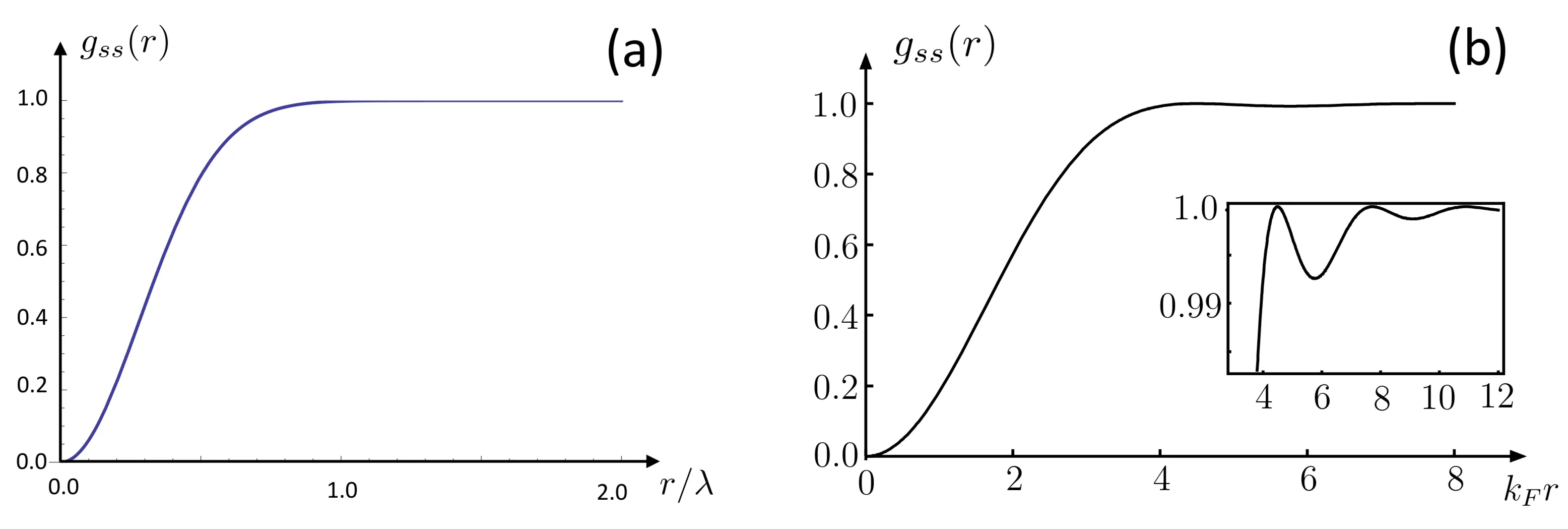
\begin{array}{r} g_{s s} (r - r^{'}) = {\begin{cases} 1 - {\frac{9 (\sin x - x \cos x)^{2}}{x^{6}} |}_{x = k_{F} | r - r^{'} |} & T = 0 \\ 1 - e^{- 2 π {(r - r^{'})}^{2} / λ^{2}} & T ≫ T_{F} . \end{cases} \end{array}

Attachments/Script 83.webp|700

The case of $s \neq s^{'}$ leads to $g_{s s^{'}} (r - r^{'}) = 1$ , meaning there is no spatial correlation between spin- $1 / 2$ fermions of opposite spin in this non-interacting model. The probability to find another fermion around the position of a fermion at $r$ corresponds to

\begin{array}{r} g (r - r^{'}) = \frac{1}{2} [g_{↑↑} (r - r^{'}) + g_{↑↓} (r - r^{'})] = \frac{1}{2} [1 - g_{s} (r - r^{'})^{2} + 1] = 1 - \frac{1}{2} g_{s} (r - r^{'})^{2} . \end{array}

The density depletion around such a fermion is then,

\begin{array}{r} \begin{aligned} n \int d^{3} R (g (R) - 1) & = - \frac{n}{2} \int d^{3} R {g_{s} (R)}^{2} \\ = - \frac{n}{2} \int d^{3} R {| \frac{2}{n} \frac{1}{V} \sum_{k} ⟨ {\hat{n}}_{k s} ⟩ e^{- i k \cdot R} |}^{2} \\ = - \frac{2}{n V} \sum_{k} {⟨ {\hat{n}}_{k s} ⟩}^{2} = {\begin{cases} - 1 & T = 0, \\ - \frac{λ^{3} n}{2^{5 / 2}} & T ≫ T_{F} . \end{cases} \end{aligned} \end{array}

which means that the exchange hole expels one fermion such that each fermion "defends" a given volume against other fermions of the same spin for $T = 0$ , while the exchange hole shrinks like $λ^{3} n$ for $T ≫ T_{F}$ .

9.6.2 Bosons

Analogous to the case of fermions, we consider first the single-particle correlation function for $s = 0$ bosons (using $\hat{a}$ for bosonic operators),

\begin{aligned} g_{1} (r - r^{'}) & = ⟨ {\hat{Ψ}}^{†} (r) \hat{Ψ} (r^{'}) ⟩ = \frac{1}{V} \sum_{k, k^{'}} e^{- i k \cdot r + i k^{'} \cdot r^{'}} ⟨ {\hat{a}}_{k}^{†} {\hat{a}}_{k^{'}} ⟩ \\ = \frac{1}{V} \sum_{k} ⟨ {\hat{n}}_{k} ⟩ e^{- i k \cdot (r - r^{'})}, \end{aligned}

which in the limit $r^{'} \to r$ approaches the constant density $n$ and vanishes at very large distances (for non-condensed systems). For $T = 0$ we consider the ground state, the Bose-Einstein condensate, $⟨ {\hat{n}}_{k} ⟩ = N δ_{k, 0}$ and for $T ≫ T_{c}$ we use the classical distribution where $T_{c}$ is the critical temperature for Bose-Einstein condensation.

\begin{array}{r} g_{1} (r - r^{'}) = {\begin{cases} n & T = 0, \\ n e^{- π {| r - r^{'} |}^{2} / λ^{2}} & T ≫ T_{c} . \end{cases} \end{array}

The pair correlation functions reads,

\begin{array}{r} \begin{aligned} g_{2} (r - r^{'}) & = ⟨ {\hat{Ψ}}^{†} (r) {\hat{Ψ}}^{†} (r^{'}) \hat{Ψ} (r^{'}) \hat{Ψ} (r) ⟩ \\ = \frac{1}{V^{2}} \sum_{k, k^{'}, q, q^{'}} e^{- i (k - k^{'}) \cdot r - i (q - q^{'}) \cdot r^{'}} ⟨ {\hat{a}}_{k}^{†} {\hat{a}}_{q}^{†} {\hat{a}}_{q^{'}} {\hat{a}}_{k^{'}} ⟩ \end{aligned} \end{array}

Analogous to the case for fermions, we evaluate the expectation value (using Wick's theorem or commutation relations for non-interacting bosons):

\begin{array}{r} ⟨ {\hat{a}}_{k}^{†} {\hat{a}}_{q}^{†} {\hat{a}}_{q^{'}} {\hat{a}}_{k^{'}} ⟩ = (1 - δ_{k q}) {δ_{k k^{'}} δ_{q q^{'}} + δ_{k q^{'}} δ_{q k^{'}}} ⟨ {\hat{n}}_{k} ⟩ ⟨ {\hat{n}}_{q} ⟩ + δ_{k q} δ_{k k^{'}} δ_{q q^{'}} (⟨ {\hat{n}}_{k}^{2} ⟩ - ⟨ {\hat{n}}_{k} ⟩) \end{array}

This leads to (after some algebra, and noting that for thermal ideal bosons $⟨ {\hat{n}}_{k}^{2} ⟩ - {⟨ {\hat{n}}_{k} ⟩}^{2} - ⟨ {\hat{n}}_{k} ⟩ (⟨ {\hat{n}}_{k} ⟩ + 1) = 0$ )

\begin{array}{r} g_{2} (r - r^{'}) = n^{2} + {| g_{1} (r - r^{'}) |}^{2} \end{array}

For $T = 0$ with $⟨ {\hat{n}}_{k} ⟩ = N δ_{k, 0}$ (so $g_{1} (r - r^{'}) = n$ ), we obtain

\begin{array}{r} g_{2} (r - r^{'}) = n^{2} + n^{2} = 2 n^{2} . \end{array}

However, a more careful evaluation for $N$ particles in a finite volume gives $g_{2} (r - r^{'}) = N (N - 1) / V^{2} = n^{2} (1 - 1 / N) \approx n^{2}$ for large $N$ . For ideal bosons in a coherent state (like a simple BEC ground state), there are no density-density correlations beyond $n^{2}$ . The result $2 n^{2}$ (or $n^{2} + | g_{1} |^{2}$ ) arises for thermal or chaotic bosonic fields. The original text's derivation for $T = 0$ :

g_{2} (r - r^{'}) = 2 n^{2} - \frac{1}{V^{2}} N (N + 1) = \frac{N (N - 1)}{V^{2}},

This implies $g_{1} (r - r^{'}) = n$ and the sum term $\frac{1}{V^{2}} \sum_{k} {⟨ {\hat{n}}_{k}^{2} ⟩ - {⟨ {\hat{n}}_{k} ⟩}^{2} - ⟨ {\hat{n}}_{k} ⟩ (⟨ {\hat{n}}_{k} ⟩ + 1)}$ evaluates to $- N (N + 1) / V^{2}$ .
This means $g_{2} (r - r^{'}) = n^{2} (1 - 1 / N)$ , which shows little spatial correlation for large $N$ .
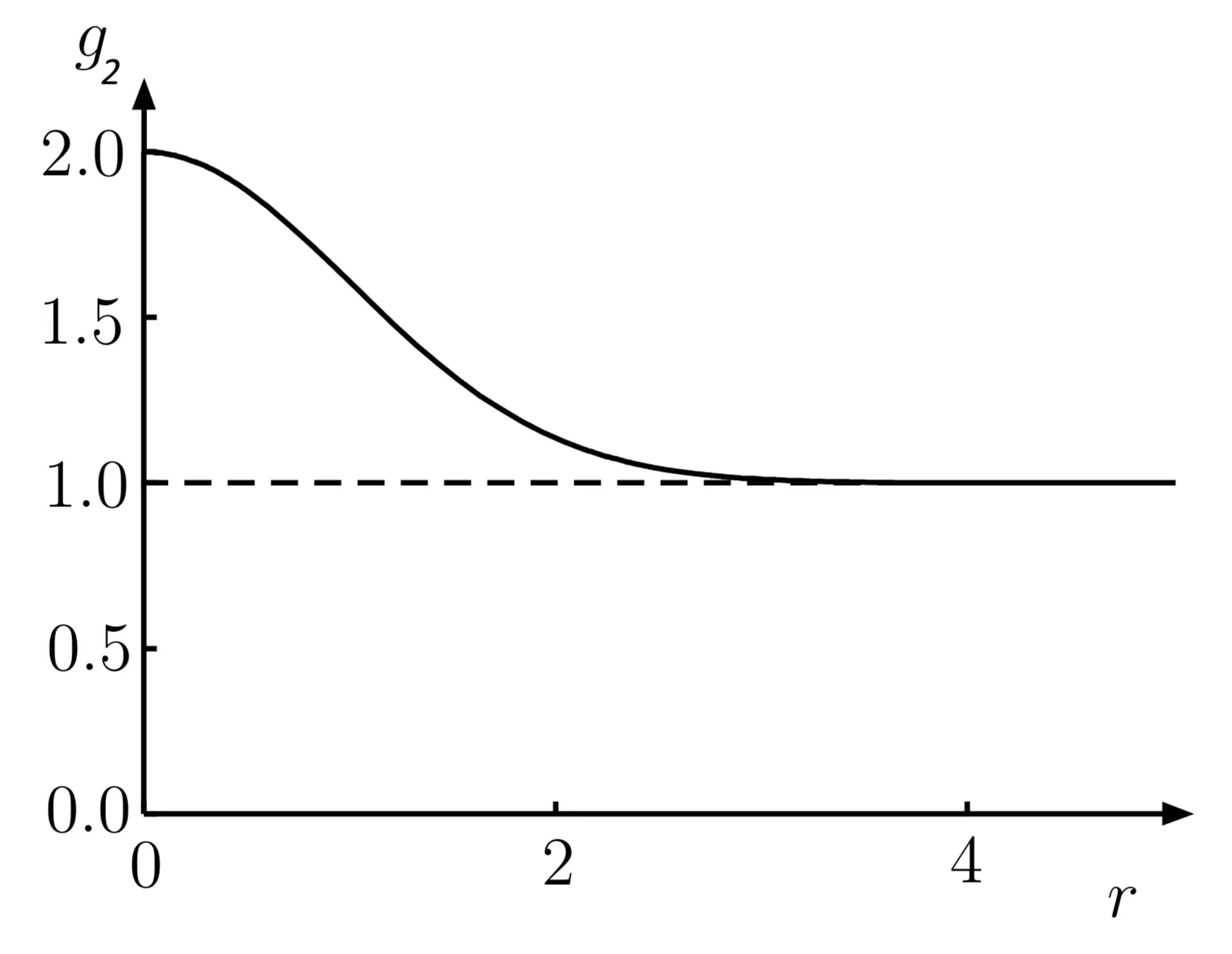
For the high-temperature limit, $T ≫ T_{c}$ , the correlation function is given

\begin{array}{r} g_{2} (r - r^{'}) = n^{2} + {| g_{1} (r - r^{'}) |}^{2} = n^{2} (1 + e^{- 2 π {| r - r^{'} |}^{2} / λ^{2}}) . \end{array}

The probability of finding two bosons at the same position ( $r = r^{'}$ ) is $g_{2} (0) = n^{2} (1 + 1) = 2 n^{2}$ , which is twice as large as for long distances ( $g_{2} (\infty) = n^{2}$ ):

Attachments/Script 84.webp|700

Thus, in contrast to fermions, bosons like to cluster together (bunching).
The radius of bunching of the bosons in the limit $T ≫ T_{c}$ is of order $λ$ and shrinks with increasing $T$ (classical limit).

9.7 Selected Applications

We consider here three examples applying second quantisation to statistical physics systems.

9.7.1 Spin Susceptibility

We calculate the spin susceptibility of spin- $1 / 2$ fermions using the fluctuation-dissipation relation.

\begin{array}{r} χ = \frac{1}{V k_{B} T} {⟨ {\hat{M}}_{z}^{2} ⟩ - {⟨ {\hat{M}}_{z} ⟩}^{2}} \end{array}

where (using $\hat{c}$ for fermion operators for consistency with earlier sections)

\begin{aligned} {\hat{M}}_{z} & = \frac{g μ_{B}}{ℏ} \int d^{3} r {\hat{S}}_{z} (r) = μ_{B} \sum_{k} \sum_{s s^{'}} {\hat{c}}_{k s}^{†} σ_{s s^{'}}^{z} {\hat{c}}_{k s^{'}} \\ = μ_{B} \sum_{k, s} s {\hat{c}}_{k s}^{†} {\hat{c}}_{k s} \end{aligned}

using results from the section on Observables in Second Quantisation. Moreover, $g = 2$ and $s = \pm 1$ (representing eigenvalues for spin up/down components). First we calculate the magnetisation in zero magnetic field,

\begin{array}{r} ⟨ {\hat{M}}_{z} ⟩ = μ_{B} \sum_{k, s} s ⟨ {\hat{c}}_{k s}^{†} {\hat{c}}_{k s} ⟩ = μ_{B} \sum_{k, s} s n_{k s} = 0 . \end{array}

Now we turn to

\begin{array}{r} ⟨ {\hat{M}}_{z}^{2} ⟩ = μ_{B}^{2} \sum_{k, s} \sum_{k^{'}, s^{'}} s s^{'} ⟨ {\hat{c}}_{k s}^{†} {\hat{c}}_{k s} {\hat{c}}_{k^{'} s^{'}}^{†} {\hat{c}}_{k^{'} s^{'}} ⟩, \end{array}

which we determine using a similar method as in the section on fermion correlation functions. The expectation value of four fermion operators for a non-interacting system is given by:

\begin{array}{r} ⟨ {\hat{c}}_{k s}^{†} {\hat{c}}_{k s} {\hat{c}}_{k^{'} s^{'}}^{†} {\hat{c}}_{k^{'} s^{'}} ⟩ = ⟨ {\hat{n}}_{k s} ⟩ (1 - ⟨ {\hat{n}}_{k s} ⟩) δ_{k k^{'}} δ_{s s^{'}} + ⟨ {\hat{n}}_{k s} ⟩ ⟨ {\hat{n}}_{k^{'} s^{'}} ⟩ . \end{array}

We now insert this result and obtain for $⟨ {\hat{M}}_{z}^{2} ⟩$ :
The term $\sum_{k s, k^{'} s^{'}} s s^{'} ⟨ {\hat{n}}_{k s} ⟩ ⟨ {\hat{n}}_{k^{'} s^{'}} ⟩ = (\sum_{k s} s ⟨ {\hat{n}}_{k s} ⟩) (\sum_{k^{'} s^{'}} s^{'} ⟨ {\hat{n}}_{k^{'} s^{'}} ⟩) = (⟨ {\hat{M}}_{z} ⟩ / μ_{B})^{2} = 0$ .
The remaining term is $μ_{B}^{2} \sum_{k s, k^{'} s^{'}} s s^{'} ⟨ {\hat{n}}_{k s} ⟩ (1 - ⟨ {\hat{n}}_{k s} ⟩) δ_{k k^{'}} δ_{s s^{'}} = μ_{B}^{2} \sum_{k s} s^{2} ⟨ {\hat{n}}_{k s} ⟩ (1 - ⟨ {\hat{n}}_{k s} ⟩)$ . Since $s^{2} = 1$ :

\begin{aligned} ⟨ {\hat{M}}_{z}^{2} ⟩ & = μ_{B}^{2} \sum_{k, s} ⟨ {\hat{n}}_{k s} ⟩ (1 - ⟨ {\hat{n}}_{k s} ⟩) \\ = μ_{B}^{2} \sum_{k, s} \frac{1}{e^{β (ϵ_{k} - μ)} + 1} (1 - \frac{1}{e^{β (ϵ_{k} - μ)} + 1}) \\ = μ_{B}^{2} \sum_{k, s} \frac{e^{β (ϵ_{k} - μ)}}{{(e^{β (ϵ_{k} - μ)} + 1)}^{2}} = μ_{B}^{2} \sum_{k, s} \frac{1}{4 \cosh^{2} (β (ϵ_{k} - μ) / 2)}, \end{aligned}

In the low-temperature limit this is confined to a narrow region ( $\sim k_{B} T$ ) around the Fermi energy, such that we approximate

\begin{aligned} ⟨ {\hat{M}}_{z}^{2} ⟩ & \approx μ_{B}^{2} V \int_{- \infty}^{+ \infty} d ϵ \frac{N (ϵ)}{V} \frac{1}{4 \cosh^{2} (β ϵ / 2)} \\ \approx μ_{B}^{2} N (ϵ_{F}) \int_{- \infty}^{+ \infty} d ϵ \frac{1}{4 \cosh^{2} (β ϵ / 2)} \\ = V μ_{B}^{2} k_{B} T \frac{N (ϵ_{F})}{V}, \end{aligned}

where $N (ϵ_{F}) / V$ is the density of states per unit volume at the Fermi energy (including both spin species if $N (ϵ_{F})$ is total DOS). The integral evaluates to $k_{B} T$ .
Then the spin susceptibility is given as the Pauli susceptibility,

\begin{array}{r} χ = \frac{1}{V k_{B} T} V μ_{B}^{2} k_{B} T \frac{N (ϵ_{F})}{V} = μ_{B}^{2} \frac{N (ϵ_{F})}{V} . \end{array}

For free fermions, $\frac{N (ϵ_{F})}{V} = \frac{3 n}{2 ϵ_{F}}$ (where $n = N / V$ is total density). So, $χ = μ_{B}^{2} \frac{3 n}{2 ϵ_{F}}$ .
The Pauli susceptibility is independent of temperature, because only $(N (ϵ_{F}) / V) k_{B} T$ fermions per unit volume can be spin polarised (thermal softening of the Fermi sea). Thus, the factor ${(k_{B} T)}^{- 1}$ in the fluctuation-dissipation formula is compensated.
The classical limit can be discussed using the Maxwell-Boltzmann distribution function,

\begin{array}{r} n_{k s} = \frac{n λ^{3}}{2 V} e^{- k^{2} λ^{2} / 4 π} (for distribution in k -space) \end{array}

with $λ$ as the thermal wavelength. Inserting this into the sum for $⟨ {\hat{M}}_{z}^{2} ⟩$ :

\begin{aligned} ⟨ {\hat{M}}_{z}^{2} ⟩ & = μ_{B}^{2} \sum_{k, s} n_{k s} (1 - n_{k s}) \\ \approx μ_{B}^{2} V \sum_{s} \int \frac{d^{3} k}{(2 π)^{3}} n_{k s} (assuming n_{k s} ≪ 1) \\ = μ_{B}^{2} V \sum_{s} (n / 2) = μ_{B}^{2} V n . \end{aligned}

This leads to the classical Curie susceptibility $χ = \frac{μ_{B}^{2} n}{k_{B} T}$ . The correction term in the original text arises if $n_{k s}$ is not negligible.

\begin{array}{r} χ = \frac{μ_{B}^{2} n}{k_{B} T} (1 - \frac{n λ^{3}}{2^{5 / 2}}) \end{array}

The factor $(1 - n_{k s})$ introduces the quantum correction (Pauli blocking) in the second term.

9.7.2 Bose-Einstein Condensate and Coherent States

Our aim here is to characterise the Bose-Einstein condensate further beyond what we did in the previous chapter. Here, we consider the concepts of both off-diagonal long-range order and the order parameter for the condensate. We start with the discussion of the single-particle correlation function for a homogeneous gas of spin-0 bosons in more detail than in the section on boson correlation functions,

\begin{aligned} g (r - r^{'}) & = ⟨ {\hat{Ψ}}^{†} (r) \hat{Ψ} (r^{'}) ⟩ \\ = \frac{1}{V} \sum_{k, k^{'}} ⟨ {\hat{a}}_{k}^{†} {\hat{a}}_{k^{'}} ⟩ e^{i (k^{'} \cdot r^{'} - k \cdot r)} \\ = \frac{1}{V} \sum_{k} ⟨ {\hat{n}}_{k} ⟩ e^{- i k \cdot (r - r^{'})}, \end{aligned}

where $⟨ {\hat{n}}_{k} ⟩$ is the Bose-Einstein distribution. For independent free bosons we may write

\begin{array}{r} g (R) = \frac{1}{V} \sum_{k} \frac{e^{- i k \cdot R}}{e^{β (ϵ_{k} - μ)} - 1}, \end{array}

with $ϵ_{k} = ℏ^{2} k^{2} / 2 m$ and $R = r - r^{'}$ . Let us look at the two limits $R \to 0$ and $R \to \infty$ . For the first limit we may expand

\begin{aligned} g (R) & = \frac{1}{V} \sum_{k} \frac{1 - i k \cdot R - (k \cdot R)^{2} / 2 + \dots}{e^{β (ϵ_{k} - μ)} - 1} \\ = n - \frac{1}{V} \sum_{k} \frac{(k \cdot R)^{2} / 2}{e^{β (ϵ_{k} - μ)} - 1} + \dots = n - \frac{R^{2}}{6 V} \sum_{k} \frac{k^{2}}{e^{β (ϵ_{k} - μ)} - 1} + \dots \\ = n - \frac{R^{2}}{6} {⟨ k^{2} ⟩}_{avg over occ. numbers} + \dots, \end{aligned}

where $n = N / V$ is the particle density and ${⟨ k^{2} ⟩}_{avg over occ. numbers} = \frac{1}{V} \sum_{k} \frac{k^{2}}{e^{β (ϵ_{k} - μ)} - 1}$ .
The text provides expressions for $⟨ k^{2} ⟩ = \frac{2 m}{ℏ^{2}} \frac{U_{t h}}{V}$ (where $U_{t h}$ is thermal internal energy):

\begin{array}{r} {⟨ k^{2} ⟩}_{avg} = {\begin{cases} \frac{1}{V} \sum_{k} k^{2} n_{M B} (ϵ_{k}) \sim 6 π n λ^{- 2} & T ≫ T_{c} \\ \frac{1}{V} \sum_{k \neq 0} k^{2} n_{B E} (ϵ_{k}) \sim 3.08 π n λ^{- 2} {(T / T_{c})}^{3 / 2} & T < T_{c} \end{cases} \end{array}

We used the average for an isotropic momentum distribution function $⟨ {\hat{n}}_{k} ⟩$ :

\begin{aligned} \frac{1}{V} \sum_{k} ⟨ (R \cdot k)^{2} {\hat{n}}_{k} ⟩ & = \frac{R^{2}}{3 V} \sum_{k} k^{2} ⟨ {\hat{n}}_{k} ⟩ = \frac{R^{2}}{3} ⟨ k^{2} ⟩_{avg} \end{aligned}

The correlation falls off quadratically for finite, but small $R (| R | ≪ λ)$ . Note that in the $T \to 0$ limit, if a condensate exists, this expansion is dominated by the $k = 0$ term for $g (R \to 0) \to n$ . For the long-distance limit ( $| R | \to \infty$ ) and $T > T_{c}$ , we note that only small wave vectors contribute significantly to the $k$ -sum so that we may expand the integrand for $β (ϵ_{k} - μ) ≪ 1$ ,

\begin{aligned} g (R) & \approx \int \frac{d^{3} k}{(2 π)^{3}} \frac{e^{- i k \cdot R}}{β (ϵ_{k} - μ)} = \frac{2 m k_{B} T}{ℏ^{2}} \int \frac{d^{3} k}{(2 π)^{3}} \frac{e^{- i k \cdot R}}{k^{2} + k_{0}^{2}} \end{aligned}

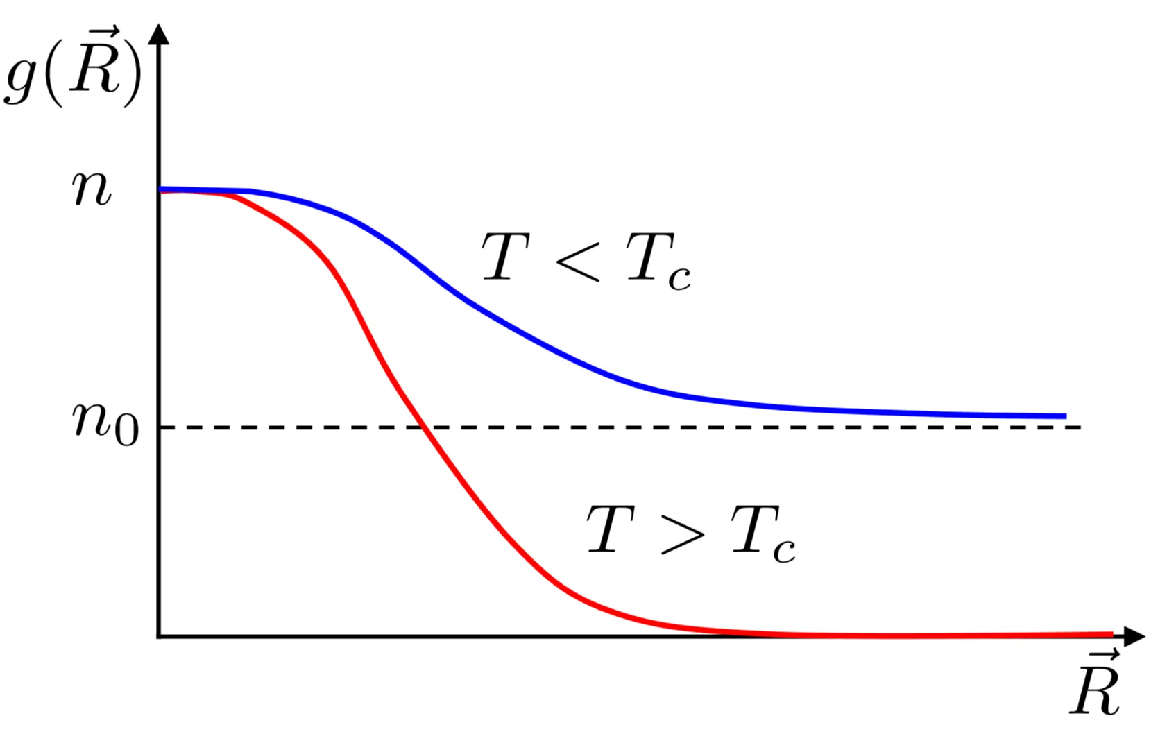
where $k_{0}^{2} = - \frac{2 m μ}{ℏ^{2}} > 0$ (since $μ < 0$ for $T > T_{c}$ ). This integral is known from the Yukawa potential, $\int \frac{d^{3} k}{(2 π)^{3}} \frac{e^{- i k \cdot R}}{k^{2} + k_{0}^{2}} = \frac{e^{- k_{0} R}}{4 π R}$ .

\begin{aligned} g (R) & \approx \frac{2 m k_{B} T}{ℏ^{2}} \frac{1}{(2 π)^{3}} \frac{e^{- k_{0} | R |}}{4 π | R |} = \frac{1}{4 π λ^{2}} \frac{e^{- k_{0} | R |}}{| R |} \end{aligned}

The single-particle correlation function decays exponentially for large distances:

Attachments/Script 85.webp|700

This behaviour is valid for $T > T_{c}$ where $μ < 0$ . For $T < T_{c}$ the chemical potential lies at the lowest single-particle state, meaning $μ = 0$ for free bosons, such that $k_{0} = 0$ . For the long-distance behaviour, the above integral would suggest $g (R) \sim 1 / | R |$ . However, this is not true, since our integral approach for $T < T_{c}$ must explicitly account for the macroscopic occupation of the $k = 0$ state. Thus, we should use

\begin{array}{r} \frac{1}{V} ⟨ {\hat{n}}_{k} ⟩ = n_{0} δ_{k, 0} + \frac{1}{V (2 π)^{3}} \frac{1}{e^{β ϵ_{k}} - 1} (for k \neq 0) \end{array}

such that for $| R | \to \infty$ , the contribution from $k \neq 0$ terms (which decay) becomes negligible compared to the $k = 0$ term:

\begin{array}{r} g (R) = \frac{1}{V} n_{0} V e^{- i 0 \cdot R} + (decaying part) \to n_{0} \end{array}

The correlation function approaches a finite value $n_{0}$ (condensate density) at long distances in the presence of a Bose-Einstein condensate. This is called off-diagonal long-range order.

Bogoliubov Approximation:

We consider this now from the viewpoint of the field operator for free bosons,

\begin{aligned} \hat{Ψ} (r) & = \frac{1}{\sqrt{V}} \sum_{k} {\hat{a}}_{k} e^{i k \cdot r} \\ = \frac{{\hat{a}}_{0}}{\sqrt{V}} + \frac{1}{\sqrt{V}} \sum_{k \neq 0} {\hat{a}}_{k} e^{i k \cdot r} \end{aligned}

The correlation function suggests the following approximation for a Bose-Einstein condensate: replace the operator ${\hat{a}}_{0}$ by a complex number (c-number), $a_{0} = \sqrt{N_{0}} e^{i ϕ}$ . Thus,

\begin{array}{r} \hat{Ψ} (r) \to ψ_{0} (r) + δ \hat{Ψ} (r), \end{array}

with $ψ_{0} (r) = \frac{a_{0}}{\sqrt{V}} = \sqrt{n_{0}} e^{i ϕ}$ , where $ϕ$ is an arbitrary phase and $n_{0} = N_{0} / V$ . In a uniform system this phase does not affect the physical properties. This so-called Bogoliubov approximation is, of course, incompatible with the occupation number representation (which assumes a fixed particle number). On the other hand, it is possible for a condensate state whose particle number is not fixed. Indeed a state incorporating this property is a coherent state.

Coherent State:

We introduce a coherent state as an eigenstate of the annihilation operator ${\hat{a}}_{ν}$ of a bosonic state of energy $ϵ_{ν}$ . Let us call this state $| Ψ_{α} ⟩$ with the property,

\begin{array}{r} {\hat{a}}_{ν} | Ψ_{α} ⟩ = α | Ψ_{α} ⟩ \end{array}

where $α$ is a complex number. Such a state is given by

\begin{array}{r} | Ψ_{α} ⟩ = e^{- | α |^{2} / 2} \sum_{N_{ν} = 0}^{\infty} \frac{α^{N_{ν}}}{\sqrt{N_{ν}!}} | N_{ν} ⟩; \end{array}

with ${\hat{a}}_{ν} | N_{ν} ⟩ = \sqrt{N_{ν}} | N_{ν} - 1 ⟩$ . The expectation value for ${\hat{n}}_{ν} = {\hat{a}}_{ν}^{†} {\hat{a}}_{ν}$ is

\begin{aligned} ⟨ {\hat{n}}_{ν} ⟩ & = ⟨ Ψ_{α} | {\hat{a}}_{ν}^{†} {\hat{a}}_{ν} | Ψ_{α} ⟩ = ⟨ Ψ_{α} | α^{*} α | Ψ_{α} ⟩ \\ = α^{*} α = | α |^{2} \end{aligned}

and the variance is

\begin{aligned} ⟨ {\hat{n}}_{ν}^{2} ⟩ - {⟨ {\hat{n}}_{ν} ⟩}^{2} & = ⟨ {\hat{a}}_{ν}^{†} {\hat{a}}_{ν} {\hat{a}}_{ν}^{†} {\hat{a}}_{ν} ⟩ - | α |^{4} \\ = ⟨ {\hat{a}}_{ν}^{†} ({\hat{a}}_{ν}^{†} {\hat{a}}_{ν} + 1) {\hat{a}}_{ν} ⟩ - | α |^{4} \\ = ⟨ {\hat{a}}_{ν}^{†} {\hat{a}}_{ν}^{†} {\hat{a}}_{ν} {\hat{a}}_{ν} ⟩ + ⟨ {\hat{a}}_{ν}^{†} {\hat{a}}_{ν} ⟩ - | α |^{4} \\ = | α |^{2} \cdot | α |^{2} + | α |^{2} - | α |^{4} = | α |^{2} \end{aligned}

such that

\begin{array}{r} \frac{\sqrt{⟨ {\hat{n}}_{ν}^{2} ⟩ - {⟨ {\hat{n}}_{ν} ⟩}^{2}}}{⟨ {\hat{n}}_{ν} ⟩} = \frac{\sqrt{| α |^{2}}}{| α |^{2}} = \frac{1}{| α |} = \frac{1}{\sqrt{⟨ {\hat{n}}_{ν} ⟩}} . \end{array}

Taking now the $k = 0$ state as coherent we identify

\begin{array}{r} {\hat{a}}_{0} | Ψ ⟩ = α_{0} | Ψ ⟩ with α_{0} = \sqrt{N_{0}} e^{i ϕ} . \end{array}

In this spirit we find that the mean value is

\begin{array}{r} ⟨ \hat{Ψ} (r) ⟩ = ψ_{0} (r), \end{array}

which does not vanish for the condensed state. Note, however, $⟨ {\hat{a}}_{k} ⟩ = 0$ , if $k \neq 0$ . The finite value of $⟨ {\hat{a}}_{0} ⟩$ requires states of different number of particles in the $k = 0$ state for the matrix elements making up this mean value. This is an element of spontaneous symmetry breaking. The condensate can be considered as a reservoir with on average $N_{0}$ particles ( $N_{0} ≫ 1$ ), to which we can add or from which we can remove particles without changing the properties of the system. The coherent state satisfies this condition. We also can define an order parameter characterising the condensate, the condensate wave function,

\begin{array}{r} ψ_{0} (r) = | ψ_{0} (r) | e^{i ϕ (r)} = \sqrt{n_{0}} e^{i ϕ} . \end{array}

Spontaneous symmetry breaking occurs via the (arbitrary) choice of the phase of the condensate wave function.
The number of particles and the phase $ϕ$ are conjugate in the sense that a state with fixed particle number has no definite phase and a state with
fixed phase has no definite particle number.

Phase and number operator eigenstates: We define the number operator and the phase operator and their corresponding eigenstates.

\begin{array}{r} \hat{N} | N ⟩ = N | N ⟩ and e^{i \hat{ϕ}} | ϕ ⟩ = e^{i ϕ} | ϕ ⟩ \end{array}

where the two states are connected by the Fourier transform

\begin{array}{r} | ϕ ⟩ = \frac{1}{\sqrt{2 π}} \sum_{N = 0}^{\infty} e^{i N ϕ} | N ⟩ with ⟨ N ∣ ϕ ⟩ = \frac{e^{- i N ϕ}}{\sqrt{2 π}} \end{array}

analogous to the relation between position and momentum eigenstates. In this context care has to be taken to ensure that the states $| ϕ ⟩$ form an orthonormal complete set of the Hilbert space. A way to construct this is to start with a finite-dimensional Hilbert space ${| N ⟩}$ assuming that $0 \leq N \leq L - 1 ≫ 1$ . Then we can restrict ourselves to a discrete set of phases $ϕ = ϕ_{k} = 2 π k / L$ with $k = 0, \dots, L - 1$ (analogous to wave vectors in a finite system with periodic boundary conditions). Now it is easy to see that

\begin{array}{r} ⟨ ϕ_{k} ∣ ϕ_{k^{'}} ⟩ = δ_{k, k^{'}} . \end{array}

Keeping this in mind we take the limit $L \to \infty$ .
Based on this, the above operators can be represented as

\begin{array}{r} \hat{N} = \sum_{N = 0}^{\infty} N | N ⟩ ⟨ N | and e^{i \hat{ϕ}} = \sum_{N = 0}^{\infty} | N ⟩ ⟨ N + 1 |; \end{array}

Thus for both $\hat{N}$ and $e^{i \hat{ϕ}}$ the coherent state does not represent an eigenstate, but rather represents a state best localised (minimum uncertainty product) in these conjugate bases.

First we consider the wave function of the coherent state in the number representation,

\begin{array}{r} Ψ_{N} = ⟨ N ∣ Ψ_{α} ⟩ = e^{- | α |^{2} / 2} \frac{α^{N}}{\sqrt{N!}} \end{array}

with $α = \sqrt{N_{0}} e^{i ϕ_{0}}$ . Thus, the probability for the particle number $N$ is given by a Poisson distribution:

\begin{array}{r} P_{N} = {| Ψ_{N} |}^{2} = e^{- | α |^{2}} \frac{| α |^{2 N}}{N!} = e^{- N_{0}} \frac{N_{0}^{N}}{N!} \approx \frac{1}{\sqrt{2 π N_{0}}} e^{- {(N - N_{0})}^{2} / 2 N_{0}} \end{array}

for large $N_{0}$ . On the other hand, projecting into the phase representation,

\begin{array}{r} \begin{aligned} Ψ_{ϕ} & = ⟨ ϕ ∣ Ψ_{α} ⟩ = \sum_{N = 0}^{\infty} ⟨ ϕ ∣ N ⟩ ⟨ N ∣ Ψ_{α} ⟩ \\ = \frac{e^{- | α |^{2} / 2}}{\sqrt{2 π}} \sum_{N = 0}^{\infty} \frac{α^{N} e^{- i ϕ N}}{\sqrt{N!}} = \frac{e^{- | α |^{2} / 2}}{\sqrt{2 π}} e^{α e^{- i ϕ}} \\ \approx \frac{1}{\sqrt{2 π}} \int_{0}^{\infty} d N \frac{e^{- {(N - N_{0})}^{2} / 4 N_{0}}}{{(2 π N_{0})}^{1 / 4}} e^{- i N (ϕ - ϕ_{0})} (using saddle point around N_{0}) \\ \approx {(\frac{N_{0}}{π})}^{1 / 4} e^{- N_{0} (ϕ - ϕ_{0})^{2}} (approximation for large N_{0}) \end{aligned} \end{array}

such that

\begin{array}{r} P_{ϕ} = {| ⟨ ϕ ∣ Ψ_{α} ⟩ |}^{2} \approx \sqrt{\frac{N_{0}}{π}} e^{- 2 N_{0} {(ϕ - ϕ_{0})}^{2}} . \end{array}

The Gaussian approximation is in both representations only valid if $N_{0} ≫ 1$ . The coherent state is neither an eigenstate of $\hat{N}$ nor $e^{i \hat{ϕ}}$ . But for both the distributions are well localised around the corresponding mean values, $N_{0}$ and $ϕ_{0}$ . The uncertainty relation is obtained by considering the deviations from the mean values,

\begin{array}{r} \begin{array}{l} Δ ϕ^{2} \approx \frac{1}{4 N_{0}} \\ Δ N^{2} = N_{0} (Poissonian) \end{array}} ⟹ Δ N Δ ϕ \approx \frac{1}{2} \end{array}

compatible with a commutation relation of the form $[\hat{N}, \hat{ϕ}] = i$ . (The exact value depends on how $Δ ϕ$ is defined for a periodic variable).

9.7.3 Phonons in an Elastic Medium

We consider here vibrations of an elastic medium using a simplified model of longitudinal waves only. As in a previous section (e.g. on lattice vibrations), we describe deformation of the elastic medium by means of the displacement field $u (r, t)$ . The kinetic and elastic energy are then given by

\begin{array}{r} E_{kin} = \frac{ρ_{m}}{2} \int d^{3} r {(\frac{\partial u (r, t)}{\partial t})}^{2} \end{array}

and

\begin{array}{r} E_{el} = \frac{λ_{e}}{2} \int d^{3} r (\nabla \cdot u (r, t))^{2} . \end{array}

where $ρ_{m}$ is the mass density of the medium and $λ_{e}$ denotes the elastic modulus. Note that we use a simplified elastic term which involves density fluctuations only, corresponding to $\nabla \cdot u$ , and ignores the contributions of shear distortion. These two energies are now combined to the Lagrangian $L = E_{kin} - E_{el}$ , whose variation with respect to $u (r, t)$ yields the wave equation,

\begin{array}{r} \frac{1}{c_{l}^{2}} \frac{\partial^{2}}{\partial t^{2}} u - \nabla (\nabla \cdot u) = 0 \end{array}

for longitudinal waves with the sound velocity $c_{l} = \sqrt{λ_{e} / ρ_{m}}$ . The general solution can be represented as a superposition of plane waves,

\begin{array}{r} u (r, t) = \frac{1}{\sqrt{V}} \sum_{k} e_{k} (q_{k} (t) e^{i k \cdot r} + q_{k}^{*} (t) e^{- i k \cdot r}) \end{array}

with polarisation vector $e_{k} = k / | k |$ (for longitudinal waves) and the amplitudes $q_{k} (t)$ satisfy the equation,

\begin{array}{r} \frac{d^{2}}{d t^{2}} q_{k} + ω_{k}^{2} q_{k} = 0 \end{array}

with the frequency $ω_{k} = c_{l} | k | = c_{l} k$ . We may rewrite the total energy, $E = E_{kin} + E_{el}$ , in terms of $q_{k}$ ,

\begin{array}{r} E = \sum_{k} ρ_{m} (| {\dot{q}}_{k} |^{2} + ω_{k}^{2} | q_{k} |^{2}) . \end{array}

Now we introduce new real variables (normal coordinates)

\begin{array}{r} Q_{k} = \sqrt{2 ρ_{m}} (q_{k} + q_{k}^{*}), and P_{k} = \sqrt{2 ρ_{m}} (- i ω_{k}) (q_{k} - q_{k}^{*}) = {\dot{Q}}_{k} \end{array}

(adjusting prefactors for canonical form if $q_{k}$ are complex amplitudes).
The energy becomes (schematically, sum over independent modes)

\begin{array}{r} E = \frac{1}{2} \sum_{k} (P_{k}^{2} + ω_{k}^{2} Q_{k}^{2}) . \end{array}

This corresponds to a set of independent harmonic oscillators labelled by the wave vectors $k$ , as seen in the discussion of lattice vibrations. We now turn to the step of canonical quantisation, replacing the classical variables $(Q_{k}, P_{k})$ with operators $({\hat{Q}}_{k}, {\hat{P}}_{k})$ which satisfy the standard commutation relation,

\begin{array}{r} [{\hat{Q}}_{k}, {\hat{P}}_{k^{'}}] = i ℏ δ_{k, k^{'}} \end{array}

This can be re-expressed in terms of lowering and raising operators,

\begin{aligned} {\hat{b}}_{k} & = \frac{1}{\sqrt{2 ℏ ω_{k}}} (ω_{k} {\hat{Q}}_{k} + i {\hat{P}}_{k}), \\ {\hat{b}}_{k}^{†} & = \frac{1}{\sqrt{2 ℏ ω_{k}}} (ω_{k} {\hat{Q}}_{k} - i {\hat{P}}_{k}) \end{aligned}

which obey the following commutation relations,

\begin{aligned} [{\hat{b}}_{k}, {\hat{b}}_{k^{'}}^{†}] & = δ_{k, k^{'}}, \\ [{\hat{b}}_{k}, {\hat{b}}_{k^{'}}] & = [{\hat{b}}_{k}^{†}, {\hat{b}}_{k^{'}}^{†}] = 0 . \end{aligned}

Therefore ${\hat{b}}_{k}^{†}$ and ${\hat{b}}_{k}$ can be viewed as creation and annihilation operators, respectively, for bosonic particles, called phonons. The Hamiltonian can be now written as

\begin{aligned} H & = \sum_{k} ℏ ω_{k} ({\hat{b}}_{k}^{†} {\hat{b}}_{k} + \frac{1}{2}) \\ = \sum_{k} ℏ ω_{k} ({\hat{n}}_{k} + \frac{1}{2}) \end{aligned}

whose eigenstates are given in the occupation number representation, $| n_{k_{1}}, n_{k_{2}}, \dots ⟩$ .
We can now also introduce the corresponding field operator,

\begin{array}{r} \hat{u} (r) = \frac{1}{\sqrt{V}} \sum_{k} e_{k} \sqrt{\frac{ℏ}{2 ρ_{m} ω_{k}}} [{\hat{b}}_{k} e^{i k \cdot r} + {\hat{b}}_{k}^{†} e^{- i k \cdot r}] \end{array}

which is not an eigenoperator for the occupation number states. Actually the thermal mean value of the field vanishes $⟨ \hat{u} (r) ⟩ = 0$ .

Correlation Function:
The correlation function is given by

\begin{array}{r} \begin{aligned} g (r - r^{'}) & = ⟨ \hat{u} (r) \cdot \hat{u} (r^{'}) ⟩ - ⟨ \hat{u} (r) ⟩ \cdot ⟨ \hat{u} (r^{'}) ⟩ = ⟨ \hat{u} (r) \cdot \hat{u} (r^{'}) ⟩ \\ = \frac{1}{V} \sum_{k, k^{'}} \frac{ℏ e_{k} \cdot e_{k^{'}}}{2 ρ_{m} \sqrt{ω_{k} ω_{k^{'}}}} ⟨ ({\hat{b}}_{k} e^{i k \cdot r} + {\hat{b}}_{k}^{†} e^{- i k \cdot r}) ({\hat{b}}_{k^{'}} e^{i k^{'} \cdot r^{'}} + {\hat{b}}_{k^{'}}^{†} e^{- i k^{'} \cdot r^{'}}) ⟩ \end{aligned} \end{array}

Note that

\begin{aligned} ⟨ {\hat{b}}_{k}^{†} {\hat{b}}_{k^{'}} ⟩ & = ⟨ {\hat{n}}_{k} ⟩ δ_{k, k^{'}}, \\ ⟨ {\hat{b}}_{k} {\hat{b}}_{k^{'}}^{†} ⟩ & = (1 + ⟨ {\hat{n}}_{k} ⟩) δ_{k, k^{'}}, \\ ⟨ {\hat{b}}_{k}^{†} {\hat{b}}_{k^{'}}^{†} ⟩ & = ⟨ {\hat{b}}_{k} {\hat{b}}_{k^{'}} ⟩ = 0, \end{aligned}

such that (since $e_{k} \cdot e_{- k} = - 1$ if $e_{k} = k / k$ , but for displacement correlations often one uses $e_{k} \cdot e_{k^{'}} = δ_{k k^{'}}$ or assumes specific polarization properties)

\begin{array}{r} g (r - r^{'}) = \frac{ℏ}{2 ρ_{m} V} \sum_{k} \frac{1}{ω_{k}} {(1 + ⟨ {\hat{n}}_{k} ⟩) e^{i k \cdot (r - r^{'})} + ⟨ {\hat{n}}_{k} ⟩ e^{- i k \cdot (r - r^{'})}} \end{array}

Melting:
Instead of calculating the correlation function for $r \neq r^{'}$ we now analyse the local (onsite) fluctuation, meaning $r = r^{'}$ ,

\begin{aligned} ⟨ u (r)^{2} ⟩ & = \frac{ℏ}{2 ρ_{m} V} \sum_{k} \frac{1}{ω_{k}} (1 + 2 ⟨ {\hat{n}}_{k} ⟩) \\ = \frac{ℏ}{2 ρ_{m} V} \sum_{k} \frac{1}{ω_{k}} \coth (\frac{β ℏ ω_{k}}{2}) \end{aligned}

With $ω_{k} = c_{l} k$ and the fact the number of degrees of freedom are limited, as described in the Debye model of lattice specific heat ( $k \leq k_{D}$ ), we find for 3D:

\begin{array}{r} ⟨ u (r)^{2} ⟩ = \frac{ℏ}{(2 π)^{2} ρ_{m} c_{l}} \int_{0}^{k_{D}} d k k \coth (\frac{β ℏ c_{l} k}{2}) = {\begin{cases} \frac{k_{D} k_{B} T}{2 π^{2} λ_{e}} & T ≫ Θ_{D} \\ \frac{k_{D}^{2} ℏ}{8 π^{2} ρ_{m} c_{l}} \approx \frac{k_{D} k_{B} Θ_{D}}{8 π^{2} λ_{e}} & T ≪ Θ_{D} \end{cases} \end{array}

which are at high (low) temperature thermal (quantum) fluctuations. As $u$ denotes the deviation of the position of an atom from its equilibrium position, we can apply Lindemann's criterion for melting of the system. We introduce the lattice constant $a$ with $k_{D} \approx π / a$ . If $⟨ u^{2} ⟩$ is a sizeable fraction of $a^{2}$ then a crystal would melt. Thus we define the Lindemann number $L_{m}$ with the
condition that the lattice is stable for $\sqrt{⟨ u^{2} ⟩} < L_{m} a$ . Thus we obtain a melting temperature $T_{m}$ from the high-T limit:

\begin{aligned} L_{m}^{2} & = \frac{⟨ u^{2} ⟩}{a^{2}} = \frac{k_{D} k_{B} T_{m}}{2 π^{2} λ_{e} a^{2}} \approx \frac{k_{B} T_{m}}{2 π λ_{e} a^{3}} \\ ⟹ & k_{B} T_{m} \approx 2 π λ_{e} a^{3} L_{m}^{2} = 2 π ρ_{m} a^{3} c_{l}^{2} L_{m}^{2} = 2 π M_{i} c_{l}^{2} L_{m}^{2} \end{aligned}

where $M_{i} = ρ_{m} a^{3}$ is the atomic mass per unit cell. Note that usually $L_{m} \approx 0.1$ gives a reasonable estimate for $T_{m}$ .
At sufficiently low temperature we can also observe quantum melting, which occurs due to quantum fluctuations, the zero-point motion of the atoms in a lattice. We consider $T ≪ Θ_{D}$ and fix the temperature (effectively $T \approx 0$ for quantum melting point calculation based on material parameters),

\begin{array}{r} L_{m}^{2} = \frac{⟨ u (0)^{2} ⟩}{a^{2}} = \frac{k_{D}^{2} ℏ}{8 π^{2} ρ_{m} c_{l} a^{2}} \approx \frac{ℏ}{8 ρ_{m} c_{l} a^{4}} ⟹ c_{l m} \approx \frac{ℏ}{8 ρ_{m} a^{4} L_{m}^{2}} \end{array}

which defines a critical value for the sound velocity, $c_{l m}$ . For $c_{l} > c_{l m}$ the fluctuations are small enough that lattice is stable because it is stiff enough, while for $c_{l} < c_{l m}$ the lattice is "soft" such that the zero-point motion destroys the lattice. We will see in a later chapter that $^{4}$ He shows such a quantum melting transition at very low temperature under pressure (pressure increases elastic constant and sound velocity), where the solid phase is stable at high pressure and turns into a liquid under decreasing pressure.

Lower Dimensions:
We consider the elastic medium at lower dimensions. For two dimensions, the integral becomes (density of states $\sim k d k$ ):

\begin{array}{r} ⟨ u (r)^{2} ⟩ = \frac{ℏ}{4 π c_{l} ρ_{m} (thickness)} \int_{0}^{k_{D}} d k \coth (\frac{β ℏ c_{l} k}{2}) \end{array}

and find that for all temperatures $T > 0$ the integral diverges at the lower integration boundary ("infrared divergence" due to $1 / k$ from $\coth (x) \sim 2 / x$ for small $x$ ). Only at $T = 0$ (where $\coth (x) \to 1$ ) we find

\begin{array}{r} {⟨ u (r)^{2} ⟩}_{T = 0} = \frac{ℏ k_{D}}{4 π c_{l} ρ_{m} (thickness)} \end{array}

is finite. Thus in two dimensions the lattice forming an elastic medium is only stable at zero temperature according to this model if long-wavelength fluctuations are not cut off by finite system size. However, we can still have quantum melting if the lattice becomes sufficiently soft. In one dimension, the integral becomes (density of states $\sim d k$ ):

\begin{array}{r} ⟨ u (r)^{2} ⟩ = \frac{ℏ}{2 π c_{l} ρ_{m} (Area)} \int_{0}^{k_{D}} d k \frac{1}{k} \coth (\frac{β ℏ c_{l} k}{2}), \end{array}

which (infrared) diverges at all temperatures including $T = 0$ (due to $1 / k^{2}$ at small $k$ for $T > 0$ , and $1 / k$ at $T = 0$ ). Quantum and thermal fluctuations are strong enough in one dimension to destabilise any lattice of infinite extent.