Table of Contents

8.1 Mott Transition
8.2 The Mott Insulator as a Quantum Spin System
8.3 Collective Modes - Spin Wave Excitations

8 Magnetism of Localised Moments

Up to now, we have mostly assumed that the interaction between electrons leads to secondary effects. This was, essentially, the message of the Fermi liquid theory, the standard model of condensed matter physics. There, the interactions of course renormalise the properties of a metal, but their description is still possible by using a language of nearly independent fermionic quasiparticles with a few modifications. Even in connection with the magnetism of itinerant electrons, where interactions proved to be crucial, the description was in terms of extended Bloch states. Many properties were determined by the band structure of the electrons in the lattice; the electrons were preferably described in $k$ -space.

However, in this chapter, we will consider situations where it is less clear whether we should describe the electrons in momentum or in real space. The problem becomes obvious with the following Gedanken experiment: We look at a regular lattice of H-atoms. The lattice constant should be large enough such that the atoms can be considered to be independent for now. In the ground state, each H-atom contains exactly one electron in the $1 s$ -state, which is the only atomic orbital we consider at the moment. The transfer of one electron to another atom would cost the relatively high energy of $E (H^{+}) + E (H^{-}) - 2 E (H) \sim 15 eV$ , since it corresponds to an ionisation. Therefore, the electrons remain localised on the individual H-atoms and the description of the electron states is obviously best done in real space. The reduction of the lattice constant will gradually increase the overlap of the electron wave functions of neighbouring atoms. In analogy to the $H_{2}$ molecule, the electrons can now extend over neighbouring atoms, but the cost in energy remains that of an "ionisation". Thus, transfer processes are only possible virtually; there are not yet itinerant electrons in the sense of a metal.

Attachments/Script 76.webp|700

On the other hand, we know the example of the alkali metals, which release their outermost ns-electron into an extended Bloch state and build a metallic (half-filled) band. This would actually work well for H-atoms for a sufficiently small lattice constant too. In nature, this can only be induced by enormous pressures – metallic hydrogen probably exists in the centres of the large gas planets Jupiter and Saturn due to the gravitational pressure. Obviously, a transition between the two limiting behaviours should exist. This metal-insulator transition occurs if the gain in kinetic energy surpasses the energy cost for charge transfer. The insulating side is known as a Mott insulator.
While the obviously metallic state is reliably described by the band picture and can be sufficiently well approximated by the previously discussed methods, this viewpoint becomes obsolete when approaching the metal-insulator transition. According to band theory, a half-filled band must produce a metal, which is definitely incorrect when entering the insulating side of the transition. Unfortunately, no well-controlled approximation for the description of this metal-insulator transition exists, since there are no small parameters for a perturbation theory.
Another important aspect is the fact that, in a standard Mott insulator, each atom features an electron in the outermost occupied orbital and, hence, a degree of freedom in the form of a localised spin $s = 1 / 2$ , in the simplest case. While charge degrees of freedom (motion of electrons) are frozen at low temperatures, the same does not apply to these spin degrees of freedom. Many interesting magnetic phenomena are produced by the coupling of these spins. Other, more general forms of Mott insulators exist as well, which include more complex forms of localised degrees of freedom, for instance, partially occupied degenerate orbital states.

8.1 Mott Transition

First, we investigate the metal-insulator transition. Its description is difficult, since it does not constitute a transition between an ordered and a disordered state in the usual sense. We will, however, use some simple considerations which will allow us to gain some insight into the behaviour of such systems.

8.1.1 Hubbard Model

We introduce a model, which is based on the tight-binding approximation we have introduced in chapter 1. It is inevitable to go back to a description based on a lattice and give up a continuum description. The model describes the motion of electrons, if their wave functions on neighbouring lattice sites only weakly overlap. Furthermore, the Coulomb repulsion, leading to an increase in energy if a site is doubly occupied, is taken into account. We include this with the lattice analogue of the contact interaction. The model, called the Hubbard model, has the form

\begin{array}{r} H = - t \sum_{⟨ i, j ⟩, s} ({\hat{c}}_{i s}^{†} {\hat{c}}_{j s} + h.c.) + U \sum_{i} {\hat{n}}_{i ↑} {\hat{n}}_{i ↓}, \end{array}

where we consider hopping between nearest neighbours only, via the matrix element $- t$ . Note that ${\hat{c}}_{i s}^{(†)}$ are real-space field operators on the lattice (site index $i$ ) and ${\hat{n}}_{i s} = {\hat{c}}_{i s}^{†} {\hat{c}}_{i s}$ is the density operator. We focus on half filling, $n = 1$ , one electron per site on average. There are two obvious limiting cases:

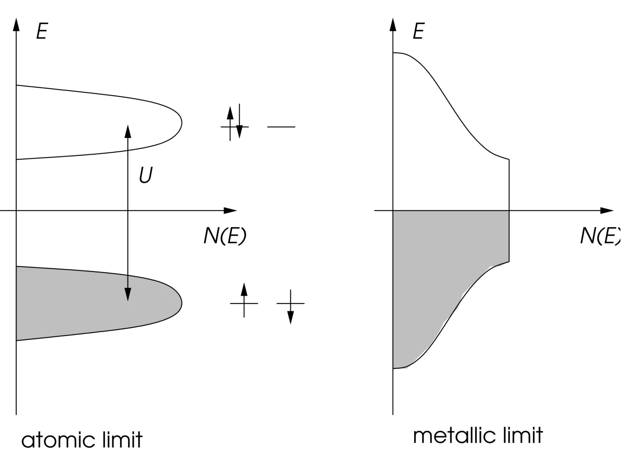
Insulating atomic limit: We put $t = 0$ . The ground state has exactly one electron on each lattice site. This state is, however, highly degenerate. In fact, the degeneracy is $2^{N}$ (number of sites $N$ ), since each electron has spin $1 / 2$ , thus,

\begin{array}{r} | Φ_{A 0} {s_{i}} ⟩ = \prod_{i} {\hat{c}}_{i, s_{i}}^{†} | 0 ⟩, \end{array}

where the spin configuration ${s_{i}}$ can be chosen arbitrarily. We will deal with the lifting of this degeneracy later. The first excited states feature one lattice site without an electron and one doubly occupied site. This state has energy $U$ and its degeneracy is even higher, namely $2^{N - 2} N (N - 1)$ . Even higher excited states correspond to more empty and doubly occupied sites. The system is an insulator and the density of states is shown here:

Attachments/Script 77.webp|700

Metallic band limit: We set $U = 0$ . The electrons are independent and move freely via hopping processes. The band energy is found through a Fourier transform of the Hamiltonian. With

\begin{array}{r} {\hat{c}}_{i s} = \frac{1}{\sqrt{N}} \sum_{k} {\hat{c}}_{k s} e^{i k \cdot r_{i}} \end{array}

we can rewrite

\begin{array}{r} - t \sum_{⟨ i, j ⟩, s} ({\hat{c}}_{i s}^{†} {\hat{c}}_{j s} + h.c.) = \sum_{k, s} ϵ_{k} {\hat{c}}_{k s}^{†} {\hat{c}}_{k s}, \end{array}

where

\begin{array}{r} ϵ_{k} = - t \sum_{a} e^{i k \cdot a} = - 2 t (\cos k_{x} a + \cos k_{y} a + \cos k_{z} a), \end{array}

and the sum runs over all vectors $a$ connecting nearest neighbours. Obviously, this system is metallic, with a unique ground state

\begin{array}{r} | Φ_{B 0} ⟩ = \prod_{k | ϵ_{k} < 0} {\hat{c}}_{k ↑}^{†} {\hat{c}}_{k ↓}^{†} | 0 ⟩ . \end{array}

Note that $ϵ_{F} = 0$ at half filling, whereas the bandwidth $2 D = 12 t$ .

8.1.2 Insulating State

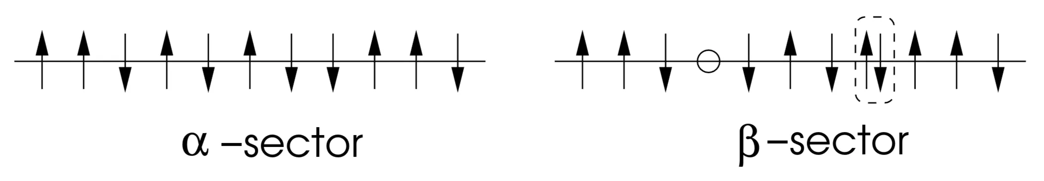
We consider the two lowest energy sectors for the case $t ≪ U$ . The ground state sector $α$ has already been defined: one electron sits on each lattice site. The lowest excited states create the sector $β$ with one empty and one doubly occupied site (as depicted in the previous figure showing the atomic limit). With the finite hopping matrix element, the empty (holon) and the doubly occupied (doublon) site become "mobile". A
fraction of the degeneracy ( $2^{N - 2} N (N - 1)$ ) is hereby lifted and the energy obtains a momentum dependence,

\begin{array}{r} E_{k, k^{'}} = U + ϵ_{k} + ϵ_{k^{'}} > U - 12 t . \end{array}

Even though ignoring the spin configurations here is a daring approximation, we obtain a qualitatively good picture of the situation. Note that the motion of an empty site (holon) or doubly occupied site (doublon) is not independent of the spin configuration which is altered by moving these objects. As a consequence, the holon/doublon motion is not entirely free leading to a reduction of the bandwidth. Therefore the bandwidth seen in the next figure is smaller than $2 D$ , in general. One notices that, with increasing $| t |$ , the two energy sectors approach each other, until they finally overlap. In the left panel the holon-doublon excitation spectrum is depicted by two bands, the lower and upper Hubbard bands, where the holon is a hole in the lower and the doublon a particle in the upper Hubbard band:

Attachments/Script 78.webp|700

The excitation gap is the gap between the two bands and we may interpret this system as an insulator, called a Mott insulator. (Note, however, that this band structure depends strongly on correlation effects, for instance, spin correlation, and is not rigid like the band structure of a semiconductor.) The band overlap (closing of the gap) indicates a transition, after which a perturbative treatment is definitely inapplicable. This is, in fact, the metal-insulator transition.

8.1.3 The Metallic State

On the metallic side, the initial state is better defined since the ground state is a filled Fermi sea without degeneracy. The treatment of the Coulomb repulsion $U$ turns out to become difficult, once we approach the Mott transition, where the electrons suffer a strong impediment in their mobility. In this region, there is no straightforward way of a perturbative treatment. The so-called Gutzwiller approximation, however, provides qualitative and very instructive insight into the properties of the strongly correlated electrons.
For this approximation we introduce the following important densities:

$1$ : electron density (average number of electrons per site, $n = 1$ for half-filling)
$s_{↑}$ : density of the singly occupied lattice sites with spin $↑$
$s_{↓}$ : density of the singly occupied lattice sites with spin $↓$
$d$ : density of the doubly occupied sites
$h$ : density of the empty sites

It is easily seen that $h = d$ and $s_{↑} = s_{↓} = s / 2$ , as long as no uniform magnetisation is present. Note that $d$ determines the energy contribution of the interaction term to $U d$ , which we regard as the index of fixed interaction energy sectors. Furthermore, for half-filling ( $n = 1$ ),

\begin{array}{r} 1 = s + 2 d \end{array}

holds. The viewpoint of the Gutzwiller approximation is based on the renormalisation of the probability of the hopping process due to the correlation of the electrons, beyond the restrictions imposed by the Pauli principle on non-interacting electrons. With this, the importance of the spatial configuration of the electrons is enhanced. In the Gutzwiller approximation, the latter is taken into account statistically by simple probabilities for the occupation of lattice sites.
We fix the density of the doubly occupied sites $d$ and investigate the hopping processes which keep $d$ constant. First, we consider an electron hopping from a singly occupied to an empty site $(i \to j)$ . Hopping probability depends on the availability of the initial configuration. We compare the probability to find this initial state for the correlated $(P)$ and the uncorrelated ( $P_{0}$ ) case and write

\begin{array}{r} P (↑ 0) + P (↓ 0) = g_{t} [P_{0} (↑ 0) + P_{0} (↓ 0)] . \end{array}

The factor $g_{t}$ will eventually appear as the renormalisation of the hopping probability and, thus, leads to an effective kinetic energy of the system due to correlations. We determine both sides statistically. In the correlated case (fixed $d$ , so $h = d$ and $s = 1 - 2 d$ ), the joint probability for $i$ to be singly occupied and $j$ to be empty is obviously

\begin{array}{r} P (↑ 0) + P (↓ 0) = s h = s d = d (1 - 2 d) . \end{array}

In the uncorrelated case (where $d$ is not fixed, and average occupancy per spin state is $1 / 2$ ), we have

\begin{aligned} P_{0} (↑ 0) = & n_{i ↑} (1 - n_{i ↓}) (1 - n_{j ↑}) (1 - n_{j ↓}) \\ = & (\frac{1}{2} \cdot \frac{1}{2}) \cdot (\frac{1}{2} \cdot \frac{1}{2}) = \frac{1}{16} . \end{aligned}

The case for $↓$ follows accordingly ( $P_{0} (↓ 0) = 1 / 16$ ). In order to collect the total result for hopping processes which keep $d$ constant, we have to do the same calculation for the hopping process $(↑↓, ↑) \to (↑, ↑↓)$ , which leads to the same result. Processes of the type $(↑↓, 0) \to (↑, ↓)$ change $d$ and are ignored for calculating $g_{t}$ . With this, we obtain in all cases the same renormalisation factor for the kinetic energy,

\begin{array}{r} g_{t} = 8 d (1 - 2 d), \end{array}

meaning, $t \to g_{t} t$ . We consider the correlations by treating the electrons as independent but with a renormalised matrix element $g_{t} t$ . The energy in the sector $d$ becomes

\begin{array}{r} E (d) = g_{t} ϵ_{kin} + U d = 8 d (1 - 2 d) ϵ_{kin} + U d, ϵ_{kin} = \frac{1}{N} \sum_{k | ϵ_{k} < 0} ϵ_{k} = \int_{- D}^{0} d ϵ N (ϵ) ϵ . \end{array}

For fixed $U$ and $t$ , we can minimise this with respect to $d$ (note that this is not a variational calculation in a strict sense, the resulting energy is not an upper bound to the ground state energy), and find

\begin{array}{r} d = \frac{1}{4} (1 - \frac{U}{U_{c}}) and g_{t} = 1 - {(\frac{U}{U_{c}})}^{2}, \end{array}

with the critical value

\begin{array}{r} U_{c} = 8 | ϵ_{kin} | \approx 25 t \sim 4 D . \end{array}

For $U \geq U_{c}$ , double occupancy and, thus, hopping is completely suppressed; electrons become localised. This observation by Brinkman and Rice provides a qualitative description of the metal-insulator transition to a Mott insulator, but takes into account only local correlations, while correlations between different lattice sites are not considered. Moreover, correlations between the spin degrees of freedom are entirely neglected. The charge excitations contain contributions between different energy scales: (1) a metallic part, described via the renormalised effective Hamiltonian

\begin{array}{r} H_{ren} = \sum_{k, s} g_{t} ϵ_{k} {\hat{c}}_{k s}^{†} {\hat{c}}_{k s} + U d, \end{array}

and (2) a part with higher energy, corresponding to charge excitations on the energy scale $U$ , meaning to excitations raising the number of doubly occupied sites by one (or more).

We can estimate the contribution to the metallic conduction. Since in the tight-binding description the current operator contains the hopping matrix element and is thus subject to the same renormalisation as the kinetic energy, we obtain

\begin{array}{r} σ_{1} (ω) = \frac{ω_{p}^{* 2}}{4 π} δ (ω) + σ_{1}^{high energy} (ω), \end{array}

where we have used the relation for a perfect conductor (no residual resistivity in a perfect lattice), as discussed in Chapter 6. There is a high-energy part which we do not specify here. The plasma frequency is renormalised, $ω_{p}^{* 2} = g_{t} ω_{p}^{2}$ , such that the $f$ -sum rule, also from Chapter 6, yields

\begin{array}{r} I = \int_{0}^{\infty} d ω σ_{1} (ω) = \frac{ω_{p}^{2}}{8 π} g_{t} + I_{high energy} = \frac{ω_{p}^{2}}{8 π} . \end{array}

For $U \to U_{c}$ , the coherent metallic part becomes weaker and weaker,

\begin{array}{r} \frac{ω_{p}^{2}}{8 π} g_{t} = (1 - {(\frac{U}{U_{c}})}^{2}) \frac{ω_{p}^{2}}{8 π} \end{array}

According to the $f$ -sum rule, the lost weight must gradually be transferred to the "high-energy" contribution.

8.1.4 Fermi Liquid Properties of the Metallic State

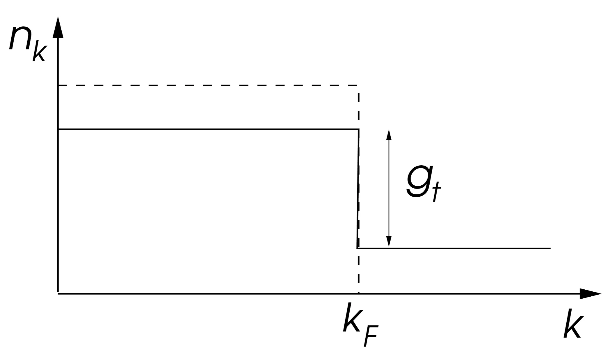
The just discussed approximation allows us to discuss a few Fermi liquid properties of the metallic state close to the metal-insulator transition in a simplified way. Let us investigate the momentum distribution. According to the above definition,

\begin{array}{r} ϵ_{kin} = \frac{1}{N} \sum_{k \in FS} ϵ_{k} \end{array}

where the sum runs over all $k$ in the Fermi sea (FS). One can show within the above approximation that the distribution is constant within ( $n_{in}$ ) and outside ( $n_{out}$ ) the Fermi surface for finite $U$ , such that, for $k$ in the first Brillouin zone,

\begin{array}{r} \frac{1}{2} = \frac{1}{N} \sum_{k \in FS} n_{in} + \frac{1}{N} \sum_{k \notin FS} n_{out} = \frac{1}{2} (n_{in} + n_{out}) \end{array}

and

\begin{array}{r} g_{t} ϵ_{kin} = \frac{1}{N} \sum_{k \in FS} n_{in} ϵ_{k} + \frac{1}{N} \sum_{k \notin FS} n_{out} ϵ_{k} . \end{array}

Taking into account particle-hole symmetry, which means

\begin{array}{r} \sum_{k} ϵ_{k} = \sum_{k \in FS} ϵ_{k} + \sum_{k \notin FS} ϵ_{k} = 0 \end{array}

we are able to determine $n_{in}$ and $n_{out}$ ,

\begin{array}{r} \begin{array}{l} n_{in} + n_{out} = 1 \\ n_{in} - n_{out} = g_{t} \end{array}} \Rightarrow {\begin{matrix} n_{in} = (1 + g_{t}) / 2 \\ n_{out} = (1 - g_{t}) / 2 \end{matrix} . \end{array}

With this, the jump in the distribution at the Fermi energy is equal to $g_{t}$ , which corresponds to the quasiparticle weight $Z$ :

Attachments/Script 79.webp|700
Quasiparticle weight $g_{t}$ as the jump in the momentum distribution.

For $U \to U_{c}$ it vanishes; the quasiparticles cease to exist for $U = U_{c}$ . Without going into the details of the calculation, we provide a few Fermi liquid parameters. It is easy to see that the effective mass ratio is

\begin{array}{r} \frac{m}{m^{*}} = g_{t} so \frac{m^{*}}{m} = g_{t}^{- 1} \end{array}

and thus

\begin{array}{r} F_{1}^{s} = 3 (\frac{m^{*}}{m} - 1) = 3 (g_{t}^{- 1} - 1) = \frac{3 U^{2}}{U_{c}^{2} - U^{2}}, \end{array}

where $t$ is related to the bare electron mass $m$ (for instance, $t \sim ℏ^{2} / (2 m a^{2})$ for a simple lattice) and the density of states $N {(ϵ_{F})}^{*} = N (ϵ_{F}) g_{t}^{- 1}$ . Furthermore,

\begin{array}{r} \begin{aligned} F_{0}^{a} = - \frac{U N (ϵ_{F})}{4} \frac{2 U_{c} + U}{{(U + U_{c})}^{2}} U_{c} ⟹ χ = \frac{μ_{B}^{2} N {(ϵ_{F})}^{*}}{1 + F_{0}^{a}} \\ F_{0}^{s} = \frac{U N (ϵ_{F})}{4} \frac{2 U_{c} - U}{{(U - U_{c})}^{2}} U_{c} ⟹ κ = \frac{N {(ϵ_{F})}^{*}}{n^{2} (1 + F_{0}^{s})} . \end{aligned} \end{array}

It follows that the compressibility $κ$ vanishes for $U \to U_{c}$ as expected, since it becomes more and more difficult to compress the electrons or to add more electrons, respectively. The insulator is, of course, incompressible. The spin susceptibility diverges because of the diverging density of states $N {(ϵ_{F})}^{*}$ . This indicates that local spins form, which exist as completely independent degrees of freedom at $U = U_{c}$ . Only the antiferromagnetic correlation between the spins would lead to a renormalisation, which turns $χ$ finite. This correlation is, as mentioned above, neglected in the Gutzwiller approximation. The effective mass diverges and shows that the quasiparticles are more and more localised close to the transition, since the occupation of a lattice site is getting more rigidly fixed to $1$ . This can be observed within the Gutzwiller approximation in the form of local fluctuations of the particle number. For this, we introduce the density matrix of the electron states on an arbitrary lattice site,

\begin{array}{r} \hat{ρ} = h | 0 ⟩ ⟨ 0 | + d | ↑↓ ⟩ ⟨ ↑↓ | + \frac{s}{2} (| ↑ ⟩ ⟨ ↑ | + | ↓ ⟩ ⟨ ↓ |) \end{array}

from which we deduce the variance of the occupation number,

\begin{array}{r} ⟨ n^{2} ⟩ - ⟨ n ⟩^{2} = ⟨ n^{2} ⟩ - 1 = tr (\hat{ρ} {\hat{n}}^{2}) - 1 = 4 d + s - 1 = 2 d . \end{array}

The deviation from single occupation vanishes with $d$ , meaning with the approach of the metal-insulator transition. Note that the fluctuation-dissipation theorem connects $⟨ n^{2} ⟩ - ⟨ n ⟩^{2}$ to the compressibility. As a last remark, it turns out that the Gutzwiller approximation is well suited to describe the strongly correlated Fermi liquid $^{3} He$ .

8.2 The Mott Insulator as a Quantum Spin System

One of the most important characteristics of the Mott insulator is the presence of spin degrees of freedom after the freezing of the charge. This is one of the most profound features distinguishing a Mott insulator from a band insulator. In our simple discussion, we have seen that the atomic limit of the Mott insulator provides us with a highly degenerate ground state, where a spin- $1 / 2$ degree of freedom is present on each lattice site. We lift this degeneracy by taking into account the kinetic energy term $H_{kin}$ (for $t ≪ U$ ). In this way new physics appears on a low-energy scale, which can be described by an effective spin Hamiltonian. Prominent examples for such spin systems are transition-metal oxides like the cuprates ${La}_{2} {CuO}_{4}, {SrCu}_{2} O_{3}$ or vanadates ${CaV}_{4} O_{9}$ , ${NaV}_{2} O_{5}$ .

8.2.1 The Effective Hamiltonian

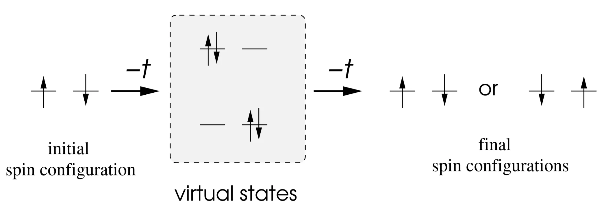
In order to employ our perturbative considerations, it is sufficient to observe the spins of two neighbouring lattice sites and to consider perturbation theory for discrete degenerate states. Here, this is preferably done in real space. There are 4 degenerate configurations, ${| ↑, ↑ ⟩, | ↑, ↓ ⟩, | ↓, ↑ ⟩, | ↓, ↓ ⟩}$ . The application of $H_{kin}$ yields

\begin{array}{r} \begin{aligned} H_{kin} | ↑, ↑ ⟩ = H_{kin} | ↓, ↓ ⟩ = 0, \\ H_{kin} | ↑, ↓ ⟩ = - t (| (↑↓)_{1}, 0_{2} ⟩ + | 0_{1}, (↑↓)_{2} ⟩), \\ H_{kin} | ↓, ↑ ⟩ = - t (| (↓↑)_{1}, 0_{2} ⟩ + | 0_{1}, (↓↑)_{2} ⟩), \end{aligned} \end{array}

where, in the last two cases, the resulting states (such as $| (↑↓)_{1}, 0_{2} ⟩$ , denoting site 1 doubly occupied and site 2 empty) have an energy higher by $U$ and lie outside the ground state sector. Thus, it becomes clear that we have to proceed to second order perturbation, where the states of higher energy will appear only virtually:

Attachments/Script 80.webp|700

We obtain the matrix elements for the effective Hamiltonian in the degenerate subspace

\begin{array}{r} M_{s_{1}, s_{2}; s_{1}^{'}, s_{2}^{'}} = - \sum_{n} ⟨ s_{1}, s_{2} | H_{kin} | n ⟩ \frac{1}{E_{n} - E_{0}} ⟨ n | H_{kin} | s_{1}^{'}, s_{2}^{'} ⟩, \end{array}

where $| n ⟩$ represents an intermediate state like $| (↑↓)_{1}, 0_{2} ⟩$ or $| 0_{1}, (↑↓)_{2} ⟩$ , such that the energy denominator $E_{n} - E_{0}$ is $U$ . We end up with (for distinct initial and final states within the ${| ↑, ↓ ⟩, | ↓, ↑ ⟩}$ subspace)

\begin{array}{r} M_{↑↓; ↑↓} = M_{↓↑; ↓↑} = - \frac{2 t^{2}}{U} and M_{↑↓; ↓↑} = M_{↓↑; ↑↓} = - \frac{2 t^{2}}{U} . \end{array}

Note that the signs originate from the anti-commutation properties of the Fermion operators during the specific evaluation of matrix elements of $H_{kin}$ . In the subspace ${| ↑, ↓ ⟩, | ↓, ↑ ⟩}$ , the Hamiltonian matrix is $(\begin{matrix} - 2 t^{2} / U & - 2 t^{2} / U \\ - 2 t^{2} / U & - 2 t^{2} / U \end{matrix})$ . The eigenstates of the respective secular equations are,

\begin{array}{r} \begin{array}{ll} \frac{1}{\sqrt{2}} (| ↑, ↓ ⟩ - | ↓, ↑ ⟩), & E = 0, \\ \frac{1}{\sqrt{2}} (| ↑, ↓ ⟩ + | ↓, ↑ ⟩), E = - \frac{4 t^{2}}{U} . \end{array} \end{array}

Since the states $| ↑, ↑ ⟩$ and $| ↓, ↓ ⟩$ have energy $E = 0$ (no hopping possible in second order that returns to these states within the degenerate manifold without changing spins), the sector with total spin $S = 1$ (triplet: $| ↑↑ ⟩, | ↓↓ ⟩, \frac{1}{\sqrt{2}} (| ↑↓ ⟩ + | ↓↑ ⟩)$ if we associate the $E = - 4 t^{2} / U$ state with the singlet and the other combinations form the triplet. This requires care: the states $| ↑↑ ⟩, | ↓↓ ⟩$ have energy $0$ . The symmetric combination $\frac{1}{\sqrt{2}} (| ↑↓ ⟩ + | ↓↑ ⟩)$ corresponds to $E = - 4 t^{2} / U$ (ground state, spin singlet $S = 0$ ). The antisymmetric combination $\frac{1}{\sqrt{2}} (| ↑↓ ⟩ - | ↓↑ ⟩)$ (part of spin triplet $S = 1$ ) has energy $0$ .
An effective Hamiltonian with the same energy spectrum for the spin configurations can be written with the help of the spin operators ${\hat{S}}_{1}$ and ${\hat{S}}_{2}$ on the two lattice sites (where $S_{i}$ are spin angular momentum operators with eigenvalues $\pm ℏ / 2$ for $S_{z}$ , and $S_{i}^{2} = S (S + 1) ℏ^{2} = (3 / 4) ℏ^{2}$ )

\begin{array}{r} H_{eff} = J ({\hat{S}}_{1} \cdot {\hat{S}}_{2} - \frac{1}{4} ℏ^{2} S (S + 1)) or more simply H_{eff} = J {\hat{S}}_{1} \cdot {\hat{S}}_{2} + const. \end{array}

Using the common form $H_{eff} = J_{exch} ({\hat{S}}_{1} \cdot {\hat{S}}_{2} / ℏ^{2})$ where $J_{exch} = - 4 t^{2} / U$ would give eigenvalues $J_{exch} (1 / 4)$ for triplet and $J_{exch} (- 3 / 4)$ for singlet.
The provided form is $H_{eff} = J ({\hat{S}}_{1} \cdot {\hat{S}}_{2} - \frac{ℏ^{2}}{4}), J = \frac{4 t^{2}}{U ℏ^{2}} > 0$ .
For $S = 1$ (triplet), $S_{1} \cdot S_{2} = ℏ^{2} / 4$ . $H_{eff} = J (ℏ^{2} / 4 - ℏ^{2} / 4) = 0$ .
For $S = 0$ (singlet), $S_{1} \cdot S_{2} = - 3 ℏ^{2} / 4$ . $H_{eff} = J (- 3 ℏ^{2} / 4 - ℏ^{2} / 4) = - J ℏ^{2} = - (4 t^{2} / U ℏ^{2}) ℏ^{2} = - 4 t^{2} / U$ . This matches the derived energies.

This mechanism of spin-spin coupling is called superexchange, a mechanism introduced by P.W. Anderson. Since this relation is valid between all neighbouring lattice sites, we can write the total Hamiltonian as

\begin{array}{r} H_{H} = J \sum_{⟨ i, j ⟩} {\hat{S}}_{i} \cdot {\hat{S}}_{j} + const. \end{array}

This model, reduced to spins only, is called the Heisenberg model. The Hamiltonian is invariant under a global $S U (2)$ spin rotation, generated by $U_{s} (θ) = e^{- i {\hat{S}}_{tot} \cdot θ / ℏ}$ , where ${\hat{S}}_{tot} = \sum_{j} {\hat{S}}_{j}$ .
Thus, the total spin is a good quantum number, as we have seen in the two-spin case. The coupling constant $J$ (as defined: $4 t^{2} / (U ℏ^{2})$ ) is positive and favors an antiparallel alignment of neighboring spins (since $S_{i} \cdot S_{j}$ is then minimized). The ground state is therefore not ferromagnetic.

8.2.2 Mean Field Approximation of the Antiferromagnet

There are a few exact results for the Heisenberg model, but not even the ground state energy can be calculated exactly (except in the case of the one-dimensional spin chain which can be solved by means of a Bethe Ansatz). The difficulty lies predominantly in the treatment of quantum fluctuations; the zero-point motion of coupled spins. It is easiest seen already with two spins, where the ground state is a singlet and maximally entangled. The ground state of all antiferromagnetic systems is a spin singlet ( $S_{tot} = 0$ ). In the so-called thermodynamic limit ( $N \to \infty$ ) there is long-range antiferromagnetic order in the ground state for dimensions $D \geq 2$ . Contrary, the fully polarised ferromagnetic state (ground state for a model with $J < 0$ ) is known exactly, and as a state with maximal spin quantum number $S_{tot}^{2}$ it features no quantum fluctuations.
In order to describe the antiferromagnetic state, we apply the mean field approximation again. We can characterise the equilibrium state of the classical Heisenberg model (spins as simple vectors without quantum properties) by splitting the lattice into two sublattices $A$ and $B$ , where each $A$ -site has only $B$ -sites as neighbors, and vice-versa. Lattices which allow for such a separation are called bipartite. There are lattices where this is not possible, for instance, triangular or face-centred cubic lattices. There, frustration phenomena appear, a further complication of antiferromagnetically coupled systems. On the $A$ - ( $B$ -) sublattice, the spins point up (down). This is unique up to a global spin rotation. Note that this spin configuration doubles the unit cell.
We introduce the respective mean field,

\begin{array}{r} {\hat{S}}_{i}^{z} \to ⟨ {\hat{S}}_{i}^{z} ⟩ = m_{i} = {\begin{cases} m & i \in A \\ - m & i \in B \end{cases} \end{array}

and the mean-field Hamiltonian on a site $i$ interacting with its $z$ neighbours $j$ is approximated by replacing terms like ${\hat{S}}_{i} \cdot {\hat{S}}_{j}$ with ${\hat{S}}_{i} \cdot ⟨ {\hat{S}}_{j} ⟩ + ⟨ {\hat{S}}_{i} ⟩ \cdot {\hat{S}}_{j} - ⟨ {\hat{S}}_{i} ⟩ \cdot ⟨ {\hat{S}}_{j} ⟩$ .
This leads to the mean field Hamiltonian

\begin{array}{r} H_{mf} = H_{A} + H_{B} = - J z m \sum_{i \in A} {\hat{S}}_{i}^{z} + J z m \sum_{i \in B} {\hat{S}}_{i}^{z} - J z \frac{m^{2}}{2} N \end{array}

with the coordination number $z$ , the number of nearest neighbors ( $z = 6$ in a simple cubic lattice). Note the constant term has been adjusted for standard mean-field derivation. It is simple to calculate the partition sum of this Hamiltonian,

\begin{array}{r} Z = tr (e^{- β H_{mf}}) = {[(2 \cosh (β J z m ℏ / 2)) e^{β J z m^{2} / 2}]}^{N} \end{array}

The free energy per spin is consequently given by

\begin{aligned} F (m, T) & = - \frac{1}{N} k_{B} T \ln Z \\ = - J z \frac{m^{2}}{2} - k_{B} T \ln (2 \cosh (β J z m ℏ / 2)) \end{aligned}

At fixed temperature, we minimise the free energy with respect to $m$ to determine the thermal equilibrium state, meaning set $\partial F / \partial m = 0$ and find

\begin{array}{r} m = \frac{ℏ}{2} \tanh (\frac{J z m ℏ}{2 k_{B} T}) \end{array}

Actually, a staggered magnetic field would be another equilibrium variable (next to the temperature). We set it to zero. This is the self-consistency equation of the mean field theory. It provides a critical temperature $T_{N}$ (Néel temperature), below which the mean moment $m$ is finite. For $T \to T_{N -}, m$ approaches 0 continuously. Thus, $T_{N}$ can be found from a linearised self-consistency equation,

\begin{array}{r} m = \frac{J z m ℏ^{2}}{4 k_{B} T_{N}} \end{array}

and thus (using $S = ℏ / 2$ )

\begin{array}{r} T_{N} = \frac{J z ℏ^{2}}{4 k_{B}} = \frac{J z (2 S)^{2}}{4 k_{B}} = \frac{J z S^{2}}{k_{B}} \end{array}

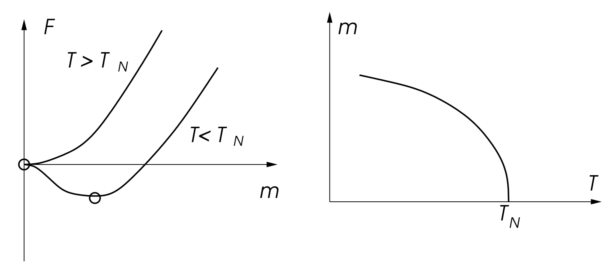
This means that $T_{N}$ scales with the coupling constant and with $z$ . The larger $J$ and the more neighbours are present, the more stable is the ordered state. At infinite $z$ , the mean field approximation becomes exact. For $T$ close to $T_{N}$ , we can expand the free energy in $m$ ,

\begin{array}{r} F (m, T) \approx F_{0} + \frac{J z}{2} [(1 - \frac{T_{N}}{T}) m^{2} + \frac{2}{3 ℏ^{2}} {(\frac{T_{N}}{T})}^{3} m^{4} \dots] \end{array}

This is a Landau theory for a phase transition of second order, where a symmetry is spontaneously broken. The breaking of the symmetry (from the high-temperature phase with high symmetry to the low-temperature phase with low symmetry) is described by the order parameter $m$ . The minimisation of $F$ with respect to $m$ yields

\begin{array}{r} m (T) \approx {\begin{cases} 0, & T > T_{N} \\ \frac{ℏ \sqrt{3}}{2} \sqrt{(1 - \frac{T}{T_{N}})}, & T ≲ T_{N} \end{cases} \end{array}

Attachments/Script 81.webp|700

8.3 Collective Modes - Spin Wave Excitations

Besides its favourable properties, the mean field approximation also has a number of insufficiencies. Quantum and some part of thermal fluctuations are neglected, and the insight into the low-energy excitations remains vague. As a matter of fact, as in the case of the ferromagnet, collective excitations exist here. In order to investigate these, we write the Heisenberg model in its spin components,

\begin{array}{r} H_{H} = J \sum_{⟨ i, j ⟩} ({\hat{S}}_{i}^{z} {\hat{S}}_{j}^{z} + \frac{1}{2} ({\hat{S}}_{i}^{+} {\hat{S}}_{j}^{-} + {\hat{S}}_{i}^{-} {\hat{S}}_{j}^{+})) . \end{array}

In the ordered state, the moments shall be aligned along the $z$ -axis.
To observe the dynamics of a flipped spin, we apply the operator $\hat{W} = \sum_{l} f_{l} {\hat{S}}_{l}^{-}$ on the ground state $| Φ_{0} ⟩$ , and determine the spectrum by solving the resulting eigenvalue equation

\begin{array}{r} (H_{H} - E_{0}) \hat{W} | Φ_{0} ⟩ = [H_{H}, \hat{W}] | Φ_{0} ⟩ = ℏ ω \hat{W} | Φ_{0} ⟩, \end{array}

with the ground state energy $E_{0}$ . Using the spin-commutation relations (for angular momentum operators $S$ including $ℏ$ )

\begin{array}{r} \begin{aligned} [{\hat{S}}_{i}^{+}, {\hat{S}}_{j}^{-}] = 2 ℏ {\hat{S}}_{i}^{z} δ_{i j}, \\ [{\hat{S}}_{i}^{z}, {\hat{S}}_{j}^{\pm}] = \pm ℏ {\hat{S}}_{j}^{\pm} δ_{i j}, \end{aligned} \end{array}

then yields the equation (after linearisation, replacing ${\hat{S}}_{j}^{z} \to ⟨ {\hat{S}}_{j}^{z} ⟩ = m_{j}$ )

\begin{array}{r} \sum_{l} [- J \sum_{j nn to l} m_{j} {\hat{S}}_{l}^{-} + J \sum_{j nn to l} m_{l} {\hat{S}}_{j}^{-} - ℏ ω {\hat{S}}_{l}^{-}] f_{l} | Φ_{0} ⟩ = 0 \end{array}

where $m_{j}$ and $m_{l}$ are the mean-field values on sites $j$ and $l$ . We decouple this complicated problem by replacing the operators ${\hat{S}}^{z}$ by their mean fields. Therefore, we have to distinguish between $A$ and $B$ sublattices ( $m_{A} = m, m_{B} = - m$ ), such that we end up with two equations,

\begin{array}{r} \begin{aligned} \sum_{l \in A} f_{l}^{A} (J m z {\hat{S}}_{l}^{-} + J m \sum_{a to nn} {\hat{S}}_{l + a}^{-} - ℏ ω {\hat{S}}_{l}^{-}) | Φ_{0} ⟩ = 0, & l \in A, \\ \sum_{l^{'} \in B} f_{l^{'}}^{B} (- J m z {\hat{S}}_{l^{'}}^{-} - J m \sum_{a to nn} {\hat{S}}_{l^{'} + a}^{-} - ℏ ω {\hat{S}}_{l^{'}}^{-}) | Φ_{0} ⟩ = 0, & l^{'} \in B . \end{aligned} \end{array}

Choosing

\begin{array}{r} \begin{aligned} f_{l}^{A} = u_{q} \sqrt{\frac{2}{N}} e^{- i q \cdot r_{l}} l \in A \\ f_{l^{'}}^{B} = v_{q} \sqrt{\frac{2}{N}} e^{- i q \cdot r_{l^{'}}} l^{'} \in B \end{aligned} \end{array}

we introduce the operators

\begin{array}{r} \begin{aligned} {\hat{a}}_{q}^{†} = \sqrt{\frac{2}{N}} \sum_{l \in A} {\hat{S}}_{l}^{-} e^{- i q \cdot r_{l}} / \sqrt{2 m ℏ} \\ {\hat{b}}_{q}^{†} = \sqrt{\frac{2}{N}} \sum_{l^{'} \in B} {\hat{S}}_{l^{'}}^{-} e^{- i q \cdot r_{l^{'}}} / \sqrt{2 m ℏ} \end{aligned} \end{array}

Inserting $f_{l}^{A}$ and $f_{l^{'}}^{B}$ into the equations of motion and using the definitions for ${\hat{a}}_{q}^{†}$ and ${\hat{b}}_{q}^{†}$ (as Fourier sums of ${\hat{S}}^{-}$ operators) leads to:

\begin{array}{r} \begin{aligned} ((J m z - ℏ ω) u_{q} + J m γ_{q} v_{q}) {\hat{A}}_{q}^{†} | Φ_{0} ⟩ = 0 \\ (- J m γ_{q} u_{q} + (- J m z - ℏ ω) v_{q}) {\hat{B}}_{q}^{†} | Φ_{0} ⟩ = 0 \end{aligned} \end{array}

where ${\hat{A}}_{q}^{†}$ and ${\hat{B}}_{q}^{†}$ represent the sums of spin operators for sublattices A and B respectively, and $γ_{q} = \sum_{a} e^{i q \cdot a} = 2 (\cos q_{x} a + \cos q_{y} a + \cos q_{z} a)$ for a simple cubic lattice. For a non-trivial solution $(u_{q}, v_{q})$ , the determinant must vanish:

| \begin{matrix} J m z - ℏ ω & J m γ_{q} \\ - J m γ_{q} & - J m z - ℏ ω \end{matrix} | = 0

This eigenvalue equation is easily solved leading to the description of spin waves in the antiferromagnet. The energy spectrum is given by

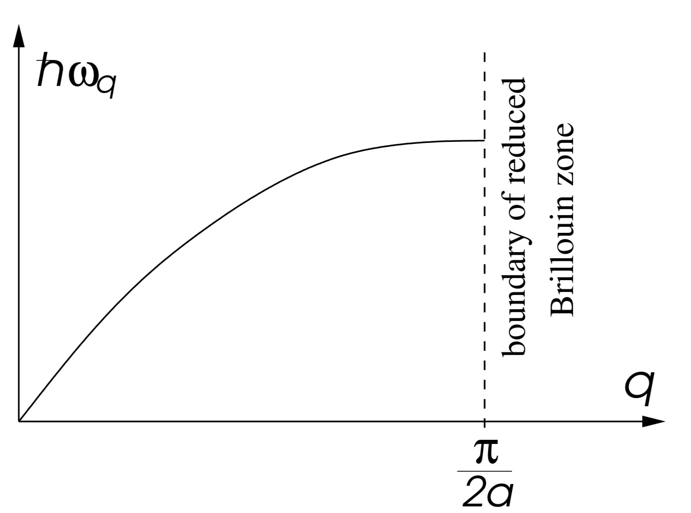
\begin{array}{r} (ℏ ω_{q})^{2} = (J m z)^{2} - (J m γ_{q})^{2} ⟹ ℏ ω_{q} = J m \sqrt{z^{2} - γ_{q}^{2}} \end{array}

Note that only the positive energies make physical sense. It is interesting to investigate the limit of small $q$ , where $γ_{q} \approx z - C q^{2}$ for some constant $C$ .
Then $z^{2} - γ_{q}^{2} \approx z^{2} - (z - C q^{2})^{2} \approx 2 z C q^{2}$ .

\begin{array}{r} ℏ ω_{q} \approx J m \sqrt{2 z C} | q | + \dots \end{array}

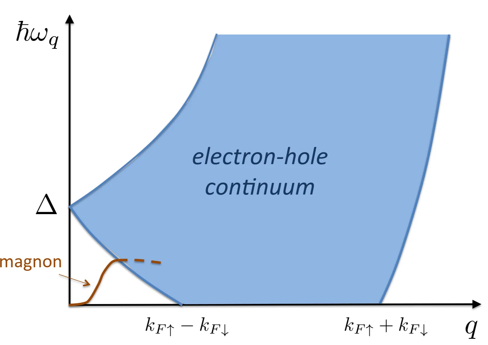
This means that, in contrast to the ferromagnet, the spin waves of the antiferromagnet have a linear low-energy spectrum (as shown in the figure below). The same applies here if we expand the spectrum around $Q = (1, 1, 1) π / a$ (folding of the Brillouin zone due to the doubling of the unit cell). After a suitable normalisation, the operators ${\hat{a}}_{q}$ and ${\hat{b}}_{q}$ (or their Bogoliubov-transformed combinations) are of bosonic nature. This is an approximation where spin operators are treated as bosons, often via Holstein-Primakoff transformation, especially for small deviations from the ordered state. For instance, $[{\hat{S}}_{l}^{+}, {\hat{S}}_{j}^{-}] = 2 ℏ {\hat{S}}_{l}^{z} δ_{l j} \approx \pm 2 ℏ m δ_{l j}$ (constant for fixed $m$ ).
The zero-point fluctuations of these bosons yield quantum fluctuations, which reduce the moment $m$ from its mean field value. In a one-dimensional spin chain these fluctuations are strong enough to suppress antiferromagnetic order even for the ground state. The fact that the spectrum starting at zero energy has to do with the infinite degeneracy of the ground state (continuous symmetry of spin rotation). This property is known under the name Goldstone theorem, which states that each ordered state resulting from the spontaneous breaking of a continuous symmetry has collective excitations with arbitrarily small (positive) energies. The linear spectrum is normal for collective excitations of this kind; the quadratic spectrum of the ferromagnet is also a Goldstone mode but with different power due to conserved total magnetisation.

Attachments/Script 82.webp|700

These spin excitations show the difference between a band and a Mott insulator very clearly. While in the band insulator both charge and spin excitations have an energy gap and are inert, the Mott insulator has only gapped charge excitations. However, the spin degrees of freedom form a low-energy sector that can even form gapless excitations, as shown above.