Table of Contents

7.1 Stoner Instability
7.2 General Spin Susceptibility and Magnetic Instabilities
7.3 Stoner Excitations

7 Magnetism in Metals

Magnetic ordering in metals can be viewed as an instability of the Fermi liquid state. We introduce this new phase of metals through the description of the Stoner ferromagnetism. The discussion of antiferromagnetism and spin density wave phases will be only brief in this chapter. In Stoner ferromagnets the magnetic moment is provided by the spin of itinerant electrons. Magnetism due to localised magnetic moments will be considered in the context of Mott insulators, which are the subject of the next chapter.
Well-known examples of elemental ferromagnetic metals are iron (Fe), cobalt (Co), and nickel (Ni) belonging to the $3 d$ transition metals, where the $3 d$ -orbital character is dominant for the conduction electrons at the Fermi energy. These orbitals are rather tightly bound to the atomic cores such that the electron mobility is reduced, enhancing the effect of interaction which is essential for the formation of a magnetic state. Other forms of magnetism, such as antiferromagnetism and the spin density wave state are found in the $3 d$ transition metals Cr and Mn. Note, $4 d$ and $5 d$ transition metals within the same columns of the periodic system are not magnetic. Their $d$ -orbitals are more extended, leading to a higher mobility of the electrons, such that the mutual interaction is insufficient to trigger magnetism. It is, however, possible to find ferromagnetism in ${ZrZn}_{2}$ where zinc (Zn) may act as a spacer reducing the mobility of the $4 d$ -electrons of zirconium (Zr). The $4 d$ -elements Pd and Rh, and the $5 d$ -element Pt are, however, nearly ferromagnetic. Going further in the periodic table, the $4 f$ -orbitals appearing in the lanthanides are nearly localised and can lead to ferromagnetism, as illustrated by the elements going from Gd through Tm in the periodic system.
Magnetism appears through a phase transition, meaning that the metal is non-magnetic at temperatures above a critical temperature $T_{c}$ , the Curie temperature. In many cases, magnetism appears at $T_{c}$ as a continuous, second order phase transition involving the spontaneous violation of symmetry. This transition is lacking latent heat (no discontinuity in entropy and volume) but instead features a discontinuity in the specific heat.

7.1 Stoner Instability

In the following section, we study the emergence of the metallic ferromagnetism originating from the Stoner mechanism. In close analogy to the first Hund's rule, the exchange interaction among the electrons plays a crucial role here. The alignment of the electronic spins in a favoured direction allows the system to reduce the energy contribution due to Coulomb repulsion. According to Landau's theory of Fermi liquids, the interaction between electrons renormalises the spin susceptibility $χ_{0}$ to

\begin{array}{r} χ = \frac{m^{*}}{m} \frac{χ_{0}}{1 + F_{0}^{a}}, \end{array}

which obviously diverges for $F_{0}^{a} \to - 1$ and leads to a ferromagnetic instability of the Fermi liquid. Then, $F_{0}^{a} \approx - U N (ϵ_{F}) / 2$ provides a critical value for the interaction $U_{c} = 2 / N (ϵ_{F})$ such that $F_{0}^{a} = - 1$ and $χ$ diverges. We will see below that this corresponds to a value we will derive also by a mean field theory.

7.1.1 Stoner Model Within the Mean Field Approximation

Consider the following model for conduction electrons with a repulsive contact interaction,

\begin{array}{r} H = \sum_{k, s} ϵ_{k} {\hat{c}}_{k s}^{†} {\hat{c}}_{k s} + U \int d^{3} r {\hat{ρ}}_{↑} (r) {\hat{ρ}}_{↓} (r), \end{array}

where we use the electron density ${\hat{ρ}}_{s} (r) = {\hat{Ψ}}_{s}^{†} (r) {\hat{Ψ}}_{s} (r)$ and the field operator ${\hat{Ψ}}_{s}^{†} ({\hat{Ψ}}_{s})$ follows from the previously established definition. The contact interaction is an approximation of the screened Coulomb interaction. Due to the Pauli exclusion principle, the contact interaction is only active between electrons with opposite spins. This is a consequence of the exchange hole in the two-particle correlation between electrons of identical spin. We obtain a useful insight into mechanisms leading to ferromagnetism by means of a mean field approximation. Note that the following mean field calculation is equivalent to a variational approach using simple many-body wave-function (Slater determinant) with different concentrations of up and down spins. We rewrite,

\begin{array}{r} {\hat{ρ}}_{s} (r) = n_{s} + [{\hat{ρ}}_{s} (r) - n_{s}], \end{array}

where

\begin{array}{r} n_{s} = ⟨ {\hat{ρ}}_{s} (r) ⟩, \end{array}

and $⟨ \cdot ⟩$ represents the thermal average. We stipulate that the deviation from the mean value $n_{s}$ is small in the sense that

\begin{array}{r} ⟨ [{\hat{ρ}}_{↑} (r) - n_{↑}] [{\hat{ρ}}_{↓} (r) - n_{↓}] ⟩ ≪ n_{↑} n_{↓} . \end{array}

Inserting this decomposition into the Hamiltonian for conduction electrons, we obtain

\begin{aligned} H_{mf} & = \sum_{k, s} ϵ_{k} {\hat{c}}_{k s}^{†} {\hat{c}}_{k s} + U \int d^{3} r [{\hat{ρ}}_{↑} (r) n_{↓} + {\hat{ρ}}_{↓} (r) n_{↑} - n_{↑} n_{↓}] \\ = \sum_{k, s} (ϵ_{k} + U n_{\bar{s}}) {\hat{c}}_{k s}^{†} {\hat{c}}_{k s} - U Ω n_{↑} n_{↓} \end{aligned}

the mean field Hamiltonian, describing electrons which move in the uniform background of electrons of opposite spin coupling via the spin dependent exchange interaction ( $\bar{s}$ denotes the spin opposite to $s$ ). Fluctuations of the form $⟨ [{\hat{ρ}}_{↑} (r) - n_{↑}] [{\hat{ρ}}_{↓} (r) - n_{↓}] ⟩$ are neglected here. The advantage of this approximation is, that the many-body problem is now reduced to an effective one-particle problem, where only the mean electron interaction is taken into account. This is equivalent to a generalised Hartree-Fock approximation and enables us to calculate certain expectation values, such as the density of one spin species, for example;

\begin{aligned} n_{↑} & = \frac{1}{Ω} \sum_{k} ⟨ {\hat{c}}_{k ↑}^{†} {\hat{c}}_{k ↑} ⟩ = \frac{1}{Ω} \sum_{k} f (ϵ_{k} + U n_{↓}) \\ = \int d ϵ \frac{1}{Ω} \sum_{k} δ (ϵ - ϵ_{k} - U n_{↓}) f (ϵ) \\ = \int d ϵ \frac{1}{2} N (ϵ - U n_{↓}) f (ϵ) \end{aligned}

where $f (ϵ)$ is the Fermi-Dirac distribution function. An analogous result is found for the opposite spin direction. These mean densities are determined self-consistently, namely such that the insertion of $n_{s}$ into the mean-field Hamiltonian provides the correct output according to the expression for $n_{↑}$ . Furthermore, the constraint that the total number of electrons is conserved, must be implemented. The real magnetisation $M = μ_{B} m$ is proportional to $m$ which is defined via

\begin{array}{r} n_{s} = \frac{1}{2} [(n_{↑} + n_{↓}) + s (n_{↑} - n_{↓})] = \frac{n_{0} + s m}{2} \end{array}

where $n_{0}$ is the total particle density and $s = \pm 1$ . This leads to the two coupled equations

\begin{aligned} n_{0} & = \frac{1}{2} \int d ϵ (N (ϵ - U n_{↓}) + N (ϵ - U n_{↑})) f (ϵ) \\ m & = \frac{1}{2} \int d ϵ (N (ϵ - U n_{↓}) - N (ϵ - U n_{↑})) f (ϵ) \end{aligned}

or equivalently

\begin{aligned} n_{0} & = \frac{1}{2} \sum_{s = \pm 1} \int d ϵ N (ϵ - \frac{U n_{0}}{2} - s \frac{U m}{2}) f (ϵ) \\ m & = - \frac{1}{2} \sum_{s = \pm 1} s \int d ϵ N (ϵ - \frac{U n_{0}}{2} - s \frac{U m}{2}) f (ϵ) \end{aligned}

which usually can not be solved analytically and must be treated numerically.

7.1.2 Stoner Criterion

An approximate solution can be found if $m ≪ n_{0}$ . The two equations are solved by adapting the chemical potential $μ$ . For low temperatures and small magnetisation we can expand $μ$ as

\begin{array}{r} μ (m, T) = ϵ_{F} + Δ μ (m, T) . \end{array}

The constant energy shift $- U n_{0} / 2$ appearing can be absorbed into $ϵ_{F}$ . The Fermi-Dirac distribution takes the form

\begin{array}{r} f (ϵ) = \frac{1}{e^{β [ϵ - μ (m, T)]} + 1} \end{array}

where $β = {(k_{B} T)}^{- 1}$ . After expanding for small $m$ , one obtains using the Sommerfeld expansion,

\begin{aligned} n_{0} & \approx \int d ϵ f (ϵ) [N (ϵ) + \frac{1}{2} {(\frac{U m}{2})}^{2} N^{''} (ϵ)] \\ \approx \int_{0}^{ϵ_{F}} d ϵ N (ϵ) + N (ϵ_{F}) Δ μ + \frac{π^{2}}{6} {(k_{B} T)}^{2} N^{'} (ϵ_{F}) + \frac{1}{2} {(\frac{U m}{2})}^{2} N^{'} (ϵ_{F}) \end{aligned}

where we introduced the abbreviations $N^{'} (ϵ) = d N (ϵ) / d ϵ$ and $N^{''} (ϵ) = d^{2} N (ϵ) / d ϵ^{2}$ . Since the first term on the right side is identical to $n_{0}$ , $Δ μ (m, T)$ is immediately found to be given by

\begin{array}{r} Δ μ (m, T) \approx - \frac{N^{'} (ϵ_{F})}{N (ϵ_{F})} [\frac{π^{2}}{6} {(k_{B} T)}^{2} + \frac{1}{2} {(\frac{U m}{2})}^{2}] . \end{array}

Analogously, the expansion of the equation for $m$ in $m$ and $T$ , results in

\begin{aligned} m & \approx \int d ϵ f (ϵ) [N^{'} (ϵ) \frac{U m}{2} + \frac{1}{3!} N^{'''} (ϵ) {(\frac{U m}{2})}^{3}] \\ \approx [N (ϵ_{F}) + \frac{π^{2}}{6} {(k_{B} T)}^{2} N^{''} (ϵ_{F}) + \frac{1}{3!} {(\frac{U m}{2})}^{2} N^{''} (ϵ_{F}) + Δ μ N^{'} (ϵ_{F})] (\frac{U m}{2}) \end{aligned}

and, finally, inserting the result for $Δ μ$ , we find

\begin{array}{r} m = N (ϵ_{F}) [1 - \frac{π^{2}}{6} {(k_{B} T)}^{2} Λ_{1}^{2} (ϵ_{F})] (\frac{U m}{2}) - N (ϵ_{F}) Λ_{2}^{2} (ϵ_{F}) {(\frac{U m}{2})}^{3} \end{array}

where

\begin{array}{r} Λ_{1}^{2} (ϵ_{F}) = {(\frac{N^{'} (ϵ_{F})}{N (ϵ_{F})})}^{2} - \frac{N^{''} (ϵ_{F})}{N (ϵ_{F})}, \end{array}

and

\begin{array}{r} Λ_{2}^{2} (ϵ_{F}) = \frac{1}{2} {(\frac{N^{'} (ϵ_{F})}{N (ϵ_{F})})}^{2} - \frac{N^{''} (ϵ_{F})}{3! N (ϵ_{F})} . \end{array}

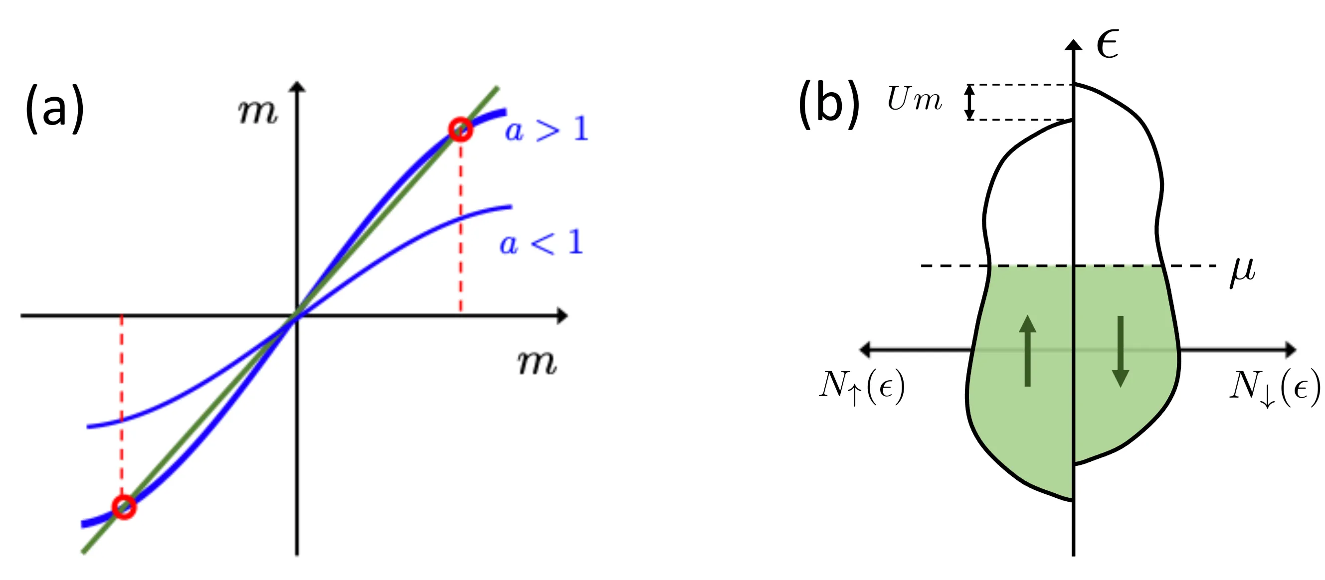
The structure is $m = a m - | b | m^{3}$ (assuming $b < 0$ for stable ferromagnetism), where $b = N (ϵ_{F}) Λ_{2}^{2} (U / 2)^{3}$ . Thus, two types of solutions emerge

\begin{array}{r} m^{2} = {\begin{cases} 0, & a < 1 \\ \frac{a - 1}{| b |}, & a \geq 1 \end{cases} \end{array}

With this, $a = 1$ corresponds to a critical value.

Attachments/Script 69.webp|700

Here, this condition corresponds to

\begin{array}{r} 1 = \frac{1}{2} U N (ϵ_{F}) [1 - \frac{π^{2}}{6} {(k_{B} T_{C})}^{2} Λ_{1}^{2} (ϵ_{F})] \end{array}

yielding

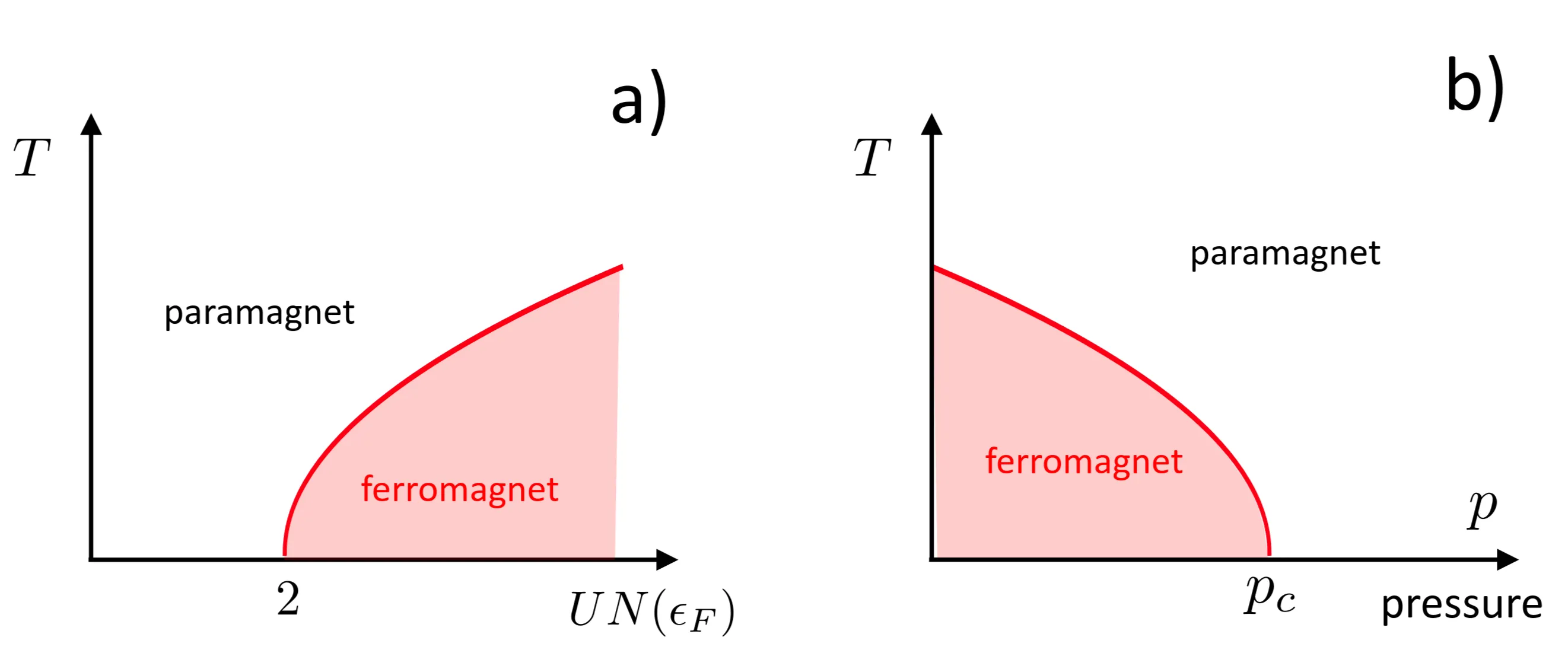
\begin{array}{r} k_{B} T_{C} = \frac{\sqrt{6}}{π Λ_{1} (ϵ_{F})} \sqrt{1 - \frac{2}{U N (ϵ_{F})}} \sim \sqrt{1 - \frac{U_{c}}{U}} \end{array}

for $U > U_{c} = 2 / N (ϵ_{F})$ . This is an instability condition for the paramagnetic Fermi liquid state with $m = 0$ , and $T_{C}$ is the Curie temperature, below which the ferromagnetic state appears. The temperature dependence of the magnetisation $M$ of the ferromagnetic state ( $T < T_{C}$ ) is given by

\begin{array}{r} M (T) = μ_{B} m (T) \sim \sqrt{T_{C} - T} \end{array}

close to the phase transition $(T_{C} - T ≪ T_{C})$ . Note that the Curie temperature $T_{C}$ is nonzero for $U N (ϵ_{F}) > 2$ , and $T_{C} \to 0$ in the limit $U N (ϵ_{F}) \to 2_{+}$ . For $U N (ϵ_{F}) < 2$ no phase transition occurs. This condition for a finite transition temperature $T_{C}$ is known as the Stoner criterion. This simple model also describes a so-called quantum phase transition, that is, a phase transition that appears at $T = 0$ as a function of system parameters, which in our case are the density of states $N (ϵ_{F})$ and the Coulomb repulsion $U$ . While thermal fluctuations destroy the ordered state at finite temperature via entropy increase, entropy is irrelevant at $T = 0$ . Here, the order is suppressed by quantum fluctuations (Heisenberg's uncertainty principle). At zero temperature we find for $m$ the following dependence on $U$ :

\begin{array}{r} m (U) = \frac{1}{Λ_{2} (ϵ_{F})} {(\frac{2}{U N (ϵ_{F})})}^{3 / 2} {(\frac{U N (ϵ_{F})}{2} - 1)}^{1 / 2} {(\frac{U}{2})}^{3 / 2} \end{array}

for $U > U_{c}$ and $m = 0$ for $U < U_{c}$ . The density of states as an internal parameter can, for example, be changed by applying a pressure. By reducing the lattice constant, pressure may facilitate the motion of the conduction electrons and increase the Fermi velocity. Consequently, the density of states is reduced:

Attachments/Script 70.webp|700

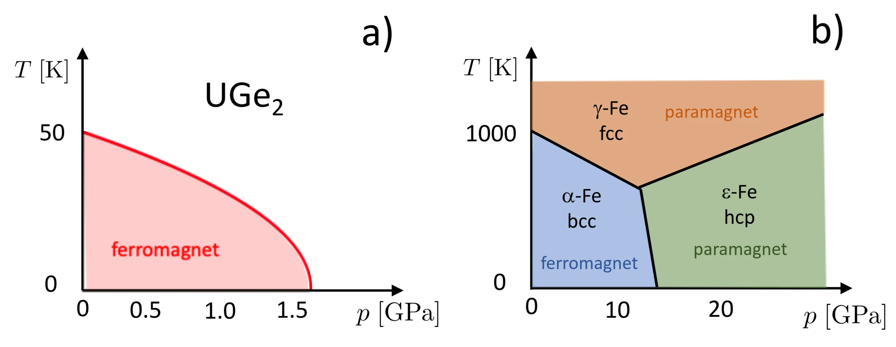
Indeed, pressure is able to destroy ferromagnetism in weakly ferromagnetic materials as ${ZrZn}_{2}$ , $MnSi$ , and ${UGe}_{2}$ . In other materials, the Curie temperature is high enough, such that the technologically applicable pressure is insufficient to suppress magnetism. It is, however, possible, that pressure leads to other transitions, such as structural phase transitions, that eventually destroy magnetism. This is seen in iron (Fe), where a pressure of about $12 GPa$ induces a transition from magnetic iron with body-centred crystal (bcc) structure to a nonmagnetic, hexagonal close packed (hcp) structure:

Attachments/Script 71.webp|700

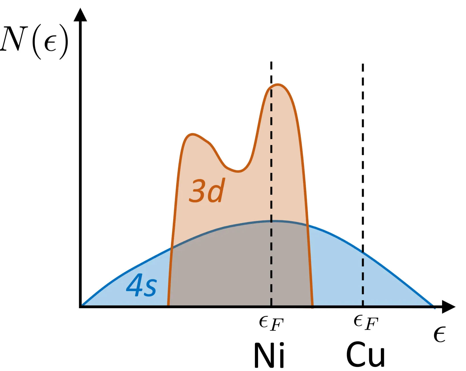
While this structural transition is a quantum phase transition as well, it appears as a discontinuous, first order transition. Note that the Stoner instability is a simplification of the quantum phase transition. In most cases, a discontinuous phase transition originates in the band structure or in fluctuation effects, which were ignored here. In some cases, pressure can also induce an increase in $N (ϵ_{F})$ , for example in metals with multiple bands, where compression leads to a redistribution of charge. One example is the ruthenate ${Sr}_{3} {Ru}_{2} O_{7}$ for which uniaxial pressure along the $z$ -axis leads to magnetism. Finally, let us turn to the question, why Cu, being a direct neighbour of Ni in the $3 d$ -row of the periodic table, is not ferromagnetic, even though both elemental metals share the same fcc crystal structure. The answer is given by the Stoner criterion $U N (ϵ_{F}) = 2$ . While the conduction electrons at the Fermi level of Ni have $3 d$ -character and belong to a narrow band with a large density of states, the Fermi energy of Cu is situated in the broad $4 s$ -band and constitutes a much smaller density of states:

Attachments/Script 72.webp|700

With this, the Cu conduction electrons are much less localised and feature a weaker tendency towards ferromagnetic order.

7.1.3 Spin Susceptibility for $T > T_{C}$

Next we study the response of the metallic system in the paramagnetic state when we apply a small magnetic field $H$ along the $z$ -axis, which induces a spin polarisation due to the Zeeman coupling,

\begin{array}{r} H_{Z} = - g μ_{B} \int d^{3} r H \frac{1}{2} {{\hat{ρ}}_{↑} (r) - {\hat{ρ}}_{↓} (r)} . \end{array}

From the self-consistency equations we obtain

\begin{aligned} m & = - \frac{1}{2} \int d ϵ f (ϵ) \sum_{s = \pm 1} s N (ϵ - μ_{B} s H - s \frac{U m}{2}) \\ \approx \int d ϵ f (ϵ) N^{'} (ϵ) (\frac{U m}{2} + μ_{B} H) \\ = N (ϵ_{F}) [1 - \frac{π^{2}}{6} {(k_{B} T)}^{2} Λ_{1} {(ϵ_{F})}^{2}] (\frac{U m}{2} + μ_{B} H) \end{aligned}

to lowest order in $m$ and $H$ . Solving this equation for $m$ yields

\begin{array}{r} M = μ_{B} m = \frac{χ_{0} (T)}{1 - U χ_{0} (T) / (2 μ_{B}^{2})} H, \end{array}

and, consequently, the magnetic susceptibility $χ$ reads

\begin{array}{r} χ = \frac{M}{H} = \frac{χ_{0} (T)}{1 - U χ_{0} (T) / (2 μ_{B}^{2})}, \end{array}

where the bare susceptibility $χ_{0}$ is given by

\begin{array}{r} χ_{0} (T) = μ_{B}^{2} N (ϵ_{F}) [1 - \frac{π^{2}}{6} {(k_{B} T)}^{2} Λ_{1} {(ϵ_{F})}^{2}] . \end{array}

We see, that the denominator of the susceptibility $χ (T)$ vanishes exactly when the Stoner instability criterion for finite temperatures is fulfilled. Thus, for $U N (ϵ_{F}) > 2$ the susceptibility

\begin{aligned} χ (T) & \approx \frac{χ_{0} (T_{C})}{(\frac{U N (ϵ_{F})}{2} - 1) (\frac{T^{2}}{T_{C}^{2}} - 1)} \\ = \frac{χ_{0} (T_{C})}{\frac{U N (ϵ_{F}) π^{2}}{12 {(k_{B} T_{C})}^{2}} {(1 - \frac{2}{U N (ϵ_{F})})}^{- 1} Λ_{1}^{2} (ϵ_{F}) k_{B}^{2} (T^{2} - T_{C}^{2})} \end{aligned}

diverging at $T_{C}$ indicates the instability. Note that for $T \to T_{C}$ from the paramagnetic side, the susceptibility diverges as $χ (T) \sim {| T_{C} - T |}^{- 1}$ corresponding to the mean field behaviour, since the mean field critical exponent $γ$ for the susceptibility takes the value $γ = 1$ .
For the case of $U N (ϵ_{F}) < 2$ there is no instability down to $T = 0$ . In the zero-temperature limit we obtain

\begin{array}{r} χ (0) = \frac{χ_{0} (0)}{1 - \frac{U N (ϵ_{F})}{2}} = \frac{μ_{B}^{2} N (ϵ_{F})}{1 + F_{0}^{a}}, \end{array}

corresponding to the form found in the Landau Fermi liquid theory with $F_{0}^{a} > - 1$ . Note that $χ_{0} (0) = μ_{B}^{2} N (ϵ_{F})$ is the Pauli spin susceptibility (assuming $g = 2$ ).

7.2 General Spin Susceptibility and Magnetic Instabilities

The ferromagnetic state is characterised by a uniform magnetisation. There are, however, magnetically ordered states which do not feature a non-zero net magnetisation but specially modulated magnetic moments. Examples are spin density wave (SDW) states, antiferromagnets and spin spiral states. In this section, we analyse general instability conditions for metallic systems towards some magnetic ordering.

7.2.1 General Dynamic Spin Susceptibility

We consider a magnetic field, oscillating in time and with spatial modulation

\begin{array}{r} H (r, t) = H_{0} e^{i q \cdot r - i ω t} e^{η t} \end{array}

where $η \to 0_{+}$ yields an adiabatic switching on of the field. We calculate the resulting magnetisation, for the corresponding Fourier component. For that, we proceed analogously to the previously discussed calculation of susceptibility and define the spin density operator $\hat{S} (r)$ in real space,

\begin{array}{r} \hat{S} (r) = \frac{ℏ}{2} \sum_{s, s^{'}} {\hat{Ψ}}_{s}^{†} (r) σ_{s s^{'}} {\hat{Ψ}}_{s^{'}} (r) = \frac{ℏ}{2} (\begin{array}{c} {\hat{Ψ}}_{↑}^{†} (r) {\hat{Ψ}}_{↓} (r) + {\hat{Ψ}}_{↓}^{†} (r) {\hat{Ψ}}_{↑} (r) \\ - i {\hat{Ψ}}_{↑}^{†} (r) {\hat{Ψ}}_{↓} (r) + i {\hat{Ψ}}_{↓}^{†} (r) {\hat{Ψ}}_{↑} (r) \\ {\hat{Ψ}}_{↑}^{†} (r) {\hat{Ψ}}_{↑} (r) - {\hat{Ψ}}_{↓}^{†} (r) {\hat{Ψ}}_{↓} (r) \end{array}) \end{array}

with momentum space representation

\begin{array}{r} {\hat{S}}_{q} = \int d^{3} r \hat{S} (r) e^{- i q \cdot r} = \frac{ℏ}{2} \sum_{k, s, s^{'}} c_{k, s}^{†} σ_{s s^{'}} c_{k + q, s^{'}} = \sum_{k} {\hat{S}}_{k, q} \end{array}

where ${\hat{S}}_{k, q} = \sum_{s, s^{'}} (ℏ / 2) c_{k, s}^{†} σ_{s s^{'}} c_{k + q, s^{'}}$ . The Hamiltonian of the electronic system with contact interaction is given by

\begin{array}{r} H = H_{0} + H_{Z} + H_{int}, \end{array}

where

\begin{array}{r} \begin{aligned} H_{0} & = \sum_{k, s} ϵ_{k} {\hat{c}}_{k s}^{†} {\hat{c}}_{k s}, \\ H_{Z} & = - \frac{g μ_{B}}{ℏ} \int d^{3} r H (r, t) \cdot \hat{S} (r), \\ H_{int} & = U \int d^{3} r {\hat{ρ}}_{↑} (r) {\hat{ρ}}_{↓} (r) . \end{aligned} \end{array}

The operator $H_{Z}$ describes the Zeeman coupling between the electrons of the metal and the perturbing field. We investigate a magnetic field

\begin{array}{r} H = H^{+} (q, ω) e^{i q \cdot r - i ω t} e^{η t} (\begin{array}{c} 1 \\ - i \\ 0 \end{array}) + h.c. \end{array}

in the $x - y$ -plane. The Zeeman term then simplifies to

\begin{array}{r} H_{Z} = - \frac{g μ_{B}}{ℏ} H^{+} (q, ω) {\hat{S}}_{- q}^{-} e^{- i ω t} e^{η t} + h.c. \end{array}

where ${\hat{S}}_{- q}^{\pm} = {\hat{S}}_{- q}^{x} \pm i {\hat{S}}_{- q}^{y}$ . In the following the Hermitian conjugate (h.c.) part will be ignored. We use

\begin{array}{r} {\hat{S}}_{- q}^{-} = ℏ \sum_{k} {\hat{c}}_{k ↓}^{†} {\hat{c}}_{k - q ↑}, \end{array}

in the $c$ -operator representation. In the framework of linear response theory, this coupling will induce a magnetisation $M_{ind}^{+} (q, t) = (μ_{B} / ℏ Ω) ⟨ {\hat{S}}_{q}^{+} (t) ⟩ \sim e^{- i ω t + η t}$ . Using a similar equation of motion formalism as used previously for charge susceptibility,

\begin{array}{r} i ℏ \frac{\partial}{\partial t} {\hat{S}}_{k, q}^{+} = [{\hat{S}}_{k, q}^{+}, H] \end{array}

with ${\hat{S}}_{k, q}^{+} = ℏ {\hat{c}}_{k ↑}^{†} {\hat{c}}_{k + q ↓}$ , we can determine this induced magnetisation, first without the interaction term $(U = 0)$ . We obtain for the given Fourier component,

\begin{array}{r} i ℏ \frac{\partial}{\partial t} {\hat{S}}_{k, q}^{+} (t) = (ϵ_{k + q} - ϵ_{k}) {\hat{S}}_{k, q}^{+} (t) - g ℏ μ_{B} (n_{k ↑} - n_{k + q ↓}) H^{+} (q, ω) e^{- i ω t + η t} \end{array}

Using the monochromatic time dependence of the field and the response $(e^{- i ω t + η t})$ and applying the thermal average we obtain,

\begin{array}{r} (ϵ_{k + q} - ϵ_{k} - ℏ ω - i ℏ η) ⟨ S_{k, q}^{+} (t) ⟩ = - g ℏ μ_{B} (n_{k + q ↑} - n_{k ↓}) H^{+} (q, ω) e^{- i ω t + η t} \end{array}

which then leads to the induced spin density-magnetisation,

\begin{array}{r} \begin{aligned} \frac{ℏ}{μ_{B}} M_{ind}^{+} (q, ω) e^{- i ω t + η t} & = \frac{1}{Ω} ⟨ S_{ind}^{+} (q, ω) ⟩ e^{- i ω t + η t} = \frac{1}{Ω} \sum_{k} ⟨ S_{k, q}^{+} (t) ⟩ \\ = \frac{ℏ}{μ_{B}} χ_{0} (q, ω) H^{+} (q, ω) e^{- i ω t + η t} \end{aligned} \end{array}

with (assuming $g = 2$ for consistency with later expressions, particularly the RPA denominator and Pauli susceptibility limit)

\begin{array}{r} χ_{0} (q, ω) = - \frac{2 μ_{B}^{2}}{Ω} \sum_{k} \frac{n_{k + q ↑} - n_{k ↓}}{ϵ_{k + q} - ϵ_{k} - ℏ ω - i ℏ η} \end{array}

Note that the form of the bare susceptibility $χ_{0} (q, ω)$ is similar to the Lindhard function, as discussed earlier in the context of charge susceptibility, actually identical, if there is no spin polarisation. This result for the induced spin density describes the induced spin density within linear response approximation.
In a next step, we want to include the effects of the interaction. Analogously to the induced charge modulation, discussed previously, the induced spin density generates an effective field on the spin of the electrons ("mean field"). The induced spin polarisation may be represented as an effective magnetic field through the exchange interaction. To implement this feature let us rewrite the contact interaction term in the form

\begin{array}{r} \begin{aligned} H_{int} & = \frac{U}{Ω} \sum_{k, k^{'}, q^{'}} {\hat{c}}_{k + q^{'} ↑}^{†} {\hat{c}}_{k ↑} {\hat{c}}_{k^{'} - q^{'} ↓}^{†} {\hat{c}}_{k^{'} ↓} \\ = - \frac{U}{2 Ω} \sum_{k, k^{'}, q^{'}} {{\hat{c}}_{k ↑}^{†} {\hat{c}}_{k + q^{'} ↓} {\hat{c}}_{k^{'} ↓}^{†} {\hat{c}}_{k^{'} - q^{'} ↑} + {\hat{c}}_{k ↓}^{†} {\hat{c}}_{k + q^{'} ↑} {\hat{c}}_{k^{'} ↑}^{†} {\hat{c}}_{k^{'} - q^{'} ↓}} + \frac{U}{Ω} \sum_{k} ({\hat{n}}_{k ↑} + {\hat{n}}_{k ↓}) \\ = - \frac{U}{2 Ω ℏ^{2}} \sum_{q^{'}} {{\hat{S}}_{q^{'}}^{+} {\hat{S}}_{- q^{'}}^{-} + {\hat{S}}_{q^{'}}^{-} {\hat{S}}_{- q^{'}}^{+}} + \frac{U}{Ω} \sum_{k} {\hat{n}}_{k} . \end{aligned} \end{array}

The last term proportional to ${\hat{n}}_{k} = {\hat{n}}_{k ↑} + {\hat{n}}_{k ↓}$ can be absorbed into the term of the chemical potential. The induced spin polarisation $⟨ S_{ind}^{+} (q, ω) ⟩$ acts through the exchange interaction as an effective (local) field, as can be seen by replacing ${\hat{S}}_{q^{'}}^{+} \to ⟨ S_{ind}^{+} (q, ω) ⟩ δ_{q, q^{'}}$ ,

\begin{array}{r} - \frac{U}{2 Ω ℏ^{2}} \sum_{q^{'}} {{\hat{S}}_{q^{'}}^{+} {\hat{S}}_{- q^{'}}^{-} + {\hat{S}}_{q^{'}}^{-} {\hat{S}}_{- q^{'}}^{+}} \to - \frac{U}{Ω ℏ^{2}} ⟨ S^{+} (q, ω) ⟩ {\hat{S}}_{- q}^{-} = - \frac{g μ_{B}}{Ω ℏ} H_{ind}^{+} (q, ω) {\hat{S}}_{- q}^{-} \end{array}

where the effective magnetic field $H_{ind}^{+} (q, ω)$ finally reads (assuming $g = 2$ for consistency with $χ_{0}$ )

\begin{array}{r} H_{ind}^{+} (q, ω) = \frac{U}{Ω g μ_{B} ℏ} ⟨ S^{+} (q, ω) ⟩ = \frac{U}{2 Ω μ_{B} ℏ} ⟨ S^{+} (q, ω) ⟩ . \end{array}

with the same monochromatic time dependence as above. This induced field acts on the spins as well, such that the total response of the spin density on the external field becomes

\begin{array}{r} \begin{aligned} M^{+} (q, ω) & = \frac{μ_{B}}{Ω ℏ} ⟨ S^{+} (q, ω) ⟩ \\ = χ_{0} (q, ω) [H^{+} (q, ω) + H_{ind}^{+} (q, ω)] \\ = χ_{0} (q, ω) H^{+} (q, ω) + χ_{0} (q, ω) \frac{U}{2 Ω μ_{B} ℏ} ⟨ S^{+} (q, ω) ⟩ \\ = χ_{0} (q, ω) H^{+} (q, ω) + χ_{0} (q, ω) \frac{U}{2 μ_{B}^{2}} M^{+} (q, ω) . \end{aligned} \end{array}

In the last step we introduce self-consistency taking the induced magnetisation as the real magnetisation. With the definition

\begin{array}{r} M^{+} (q, ω) = χ (q, ω) H^{+} (q, ω) \end{array}

of the susceptibility we find

\begin{array}{r} χ (q, ω) = \frac{χ_{0} (q, ω)}{1 - \frac{U}{2 μ_{B}^{2}} χ_{0} (q, ω)} . \end{array}

which corresponds to the random phase approximation (RPA), as discussed earlier. This form of the susceptibility is found to be valid for all field directions, as long as spin-orbit coupling is neglected. Within the random phase approximation, the generalisation of the Stoner criterion for the appearance of an instability of the system at finite temperature reads

\begin{array}{r} 1 = \frac{U}{2 μ_{B}^{2}} χ_{0} (q, ω) . \end{array}

For the limiting case $(q, ω) \to (0, 0)$ corresponding to a uniform, static external field, we obtain for the bare susceptibility

\begin{array}{r} \begin{aligned} χ_{0} (q, 0) = - \frac{2 μ_{B}^{2}}{Ω} \sum_{k} \frac{n_{k + q ↑} - n_{k ↓}}{ϵ_{k + q} - ϵ_{k}} \\ \overset{q \to 0}{\to} - \frac{2 μ_{B}^{2}}{Ω} \sum_{k} \frac{\partial f (ϵ_{k})}{\partial ϵ_{k}} = χ_{0} (T), \end{aligned} \end{array}

which corresponds to the Pauli susceptibility (with $g = 2$ ). Then, $χ (T)$ (the full susceptibility) is again cast into the form previously discussed for the simpler ferromagnetic case and describes the instability of the metal with respect to ferromagnetic spin polarisation, when the denominator vanishes. Similar to the charge density wave, the isotropic deformation for $q = 0$ is not the leading instability, when $χ_{0} (Q, 0) > χ_{0} (0, 0)$ for a finite $Q$ . Then, another form of magnetic order is more favoured.

7.2.2 Instability with Finite Wave Vector $Q$

In order to show that, indeed, the Stoner instability does not always prevail among all possible magnetic instabilities, we first go through a simple argument based on the local susceptibility. For that, we define the local magnetic moment along the $z$ -axis, $M (r) = μ_{B} ⟨ {\hat{ρ}}_{↑} (r) - {\hat{ρ}}_{↓} (r) ⟩$ , and consider the non-local relation

\begin{array}{r} M (r) = \int d^{3} r^{'} {\tilde{χ}}_{0} (r - r^{'}) H_{z} (r^{'}) \end{array}

within the linear response approximation. In Fourier space, the same relation reads

\begin{array}{r} M_{q} = χ_{0} (q) H_{q}, \end{array}

with

\begin{array}{r} χ_{0} (q) = \int d^{3} r {\tilde{χ}}_{0} (r) e^{- i q \cdot r} \end{array}

Now, compare $χ_{0} (q = 0)$ with $\overset{―}{χ_{0} (q)}$ defined as

\begin{array}{r} \overset{―}{χ_{0} (q)} = \frac{1}{Ω} \sum_{q} χ_{0} (q) = \frac{1}{Ω} \sum_{q} \int d^{3} r {\tilde{χ}}_{0} (r) e^{- i q \cdot r} = \int d^{3} r {\tilde{χ}}_{0} (r) δ (r) = {\tilde{χ}}_{0} (r = 0) \end{array}

This $q$ -averaged susceptibility corresponds to the local susceptibility. For a paramagnetic metal at $T = 0$ we may write (using a "per spin" density of states $N (ϵ)$ and corresponding susceptibility definition consistent with $χ_{0} (q = 0) = μ_{B}^{2} N (ϵ_{F})$ for this subsection's comparison):

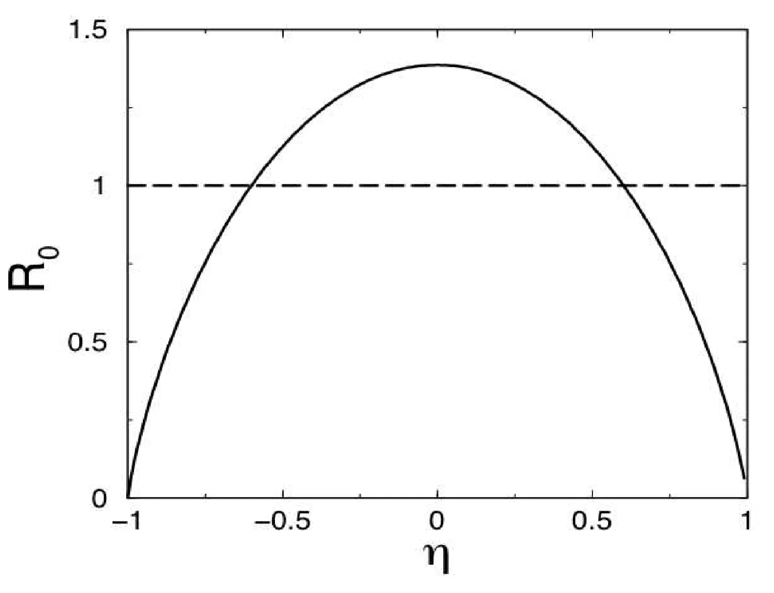
\begin{array}{r} \overset{―}{χ_{0} (q)} = \frac{2 μ_{B}^{2}}{Ω^{2}} \sum_{k, q} \frac{n_{k + q ↑} - n_{k ↓}}{ϵ_{k} - ϵ_{k + q}} = \frac{μ_{B}^{2}}{2} \int d ϵ N (ϵ) \int d ϵ^{'} N (ϵ^{'}) \frac{f (ϵ) - f (ϵ^{'})}{ϵ^{'} - ϵ}, \end{array}

and must be compared to $χ_{0} (q = 0) = μ_{B}^{2} N (ϵ_{F}) (f (ϵ) = Θ (ϵ_{F} - ϵ))$ . The local susceptibility depends on the density of states and the Fermi energy of the system. A very good qualitative understanding can be obtained by a very simple form

\begin{array}{r} N (ϵ) = {\begin{array}{lr} \frac{1}{D}, & - D \leq ϵ \leq D \\ 0, & | ϵ | > D \end{array} \end{array}

for the density of states which does not correspond to a particular band structure but mimics a band of width $2 D$ . With this rough approximation, the integral for $\overset{―}{χ_{0} (q)}$ is easily evaluated. The ratio between $\overset{―}{χ (q)}$ and $χ_{0} (q = 0)$ is then found to be

\begin{array}{r} R_{0} = \frac{\overset{―}{χ_{0} (q)}}{χ_{0} (q = 0)} = \ln (\frac{4}{1 - η^{2}}) + η \ln (\frac{1 - η}{1 + η}) \end{array}

with $η = ϵ_{F} / D$ where $- D < ϵ_{F} < + D$ . For both small and large band fillings ( $ϵ_{F}$ close to the band edges), the tendency towards ferromagnetism dominates, whereas when $ϵ_{F}$ lies in the centre of the band, the susceptibility $χ_{0} (q)$ is not maximal at $q = 0$ anymore, and magnetic ordering with a well-defined finite $q = Q$ becomes more probable.

Attachments/Script 73.webp|700

7.2.3 Influence of the Band Structure

Whether magnetic order arises at finite $q$ or not depends strongly on the details of the band structure. The argument given above, comparing the local $(r = 0)$ to the uniform $(q = 0)$ susceptibility is nothing more than a vague indicator for a possible instability at non-zero $q$ . A crucial ingredient for the appearance of magnetic order at a given $q = Q$ is the so-called nesting of the Fermi surface. Within extended areas of the Fermi surface the energy dispersion satisfies the nesting condition,

\begin{array}{r} ξ_{k + Q} = - ξ_{k} \end{array}

where $ξ_{k} = ϵ_{k} - ϵ_{F}$ and $Q$ is some fixed vector. The nesting conditions connects for given $k$ an electron- and hole-like band states (at $T = 0$ filled and empty states, respectively). If the Fermi surface of a material features such a nesting trait, the susceptibility will be dominated by the contribution from this vector $Q$ . In order to see this, let us investigate the static susceptibility $χ_{0} (q)$ for $q = Q$ under the assumption that the nesting condition holds for all $k$ (see tight-binding example below). Thus,

\begin{array}{r} χ_{0} (Q; T) = \frac{2 μ_{B}^{2}}{Ω} \sum_{k} \frac{n_{k + Q} - n_{k}}{ξ_{k} - ξ_{k + Q}} = μ_{B}^{2} \int \frac{d^{3} k}{(2 π)^{3}} \frac{\tilde{f} (- ξ_{k}) - \tilde{f} (ξ_{k})}{ξ_{k}}, \end{array}

where $\tilde{f} (ξ) = f (ξ + ϵ_{F}) = f (ϵ) = {[\exp (ξ / k_{B} T) + 1]}^{- 1}$ and $f$ is the Fermi-Dirac distribution. Under the further assumption that $ξ_{k}$ is weakly angle dependent, we find

\begin{aligned} χ_{0} (Q; T) & = μ_{B}^{2} \int \frac{d^{3} k}{(2 π)^{3}} \frac{\tanh (ξ_{k} / 2 k_{B} T)}{ξ_{k}} \\ = \frac{μ_{B}^{2}}{2} \int d ξ N (ξ + ϵ_{F}) \frac{\tanh (ξ / 2 k_{B} T)}{ξ} . \end{aligned}

In order to approximate this integral properly, we notice that the integral has a logarithmic divergence at infinite energies $ξ$ . The band width gives a natural cutoff. Let us, therefore, take the density of states with $ϵ_{F} = 0$ ,

\begin{array}{r} \begin{aligned} χ_{0} (Q; T) & \approx μ_{B}^{2} N (ϵ_{F}) \int_{0}^{ϵ_{0}} d ξ \frac{\tanh (ξ / 2 k_{B} T)}{ξ} \\ = μ_{B}^{2} N (ϵ_{F}) (\ln (\frac{ϵ_{0}}{2 k_{B} T}) + \ln (\frac{4 e^{γ}}{π})) \\ \approx μ_{B}^{2} N (ϵ_{F}) \ln (\frac{1.14 ϵ_{0}}{k_{B} T}), \end{aligned} \end{array}

where we assumed $ϵ_{0} ≫ k_{B} T$ , cutoff energy of the order of the band width, and where $γ \approx 0.57721$ is the Euler-Mascheroni constant. The bare susceptibility $χ_{0}$ diverges logarithmically at zero temperatures. Inserting this result for $χ_{0} (Q; T)$ into the generalised Stoner relation, results in

\begin{array}{r} 0 = 1 - \frac{U N (ϵ_{F})}{2} \ln (\frac{1.14 ϵ_{0}}{k_{B} T_{c}}), \end{array}

with the critical temperature

\begin{array}{r} k_{B} T_{c} = 1.14 ϵ_{0} e^{- 2 / U N (ϵ_{F})} . \end{array}

A finite critical temperature persists for arbitrarily small positive values of $U N (ϵ_{F})$ . The nesting condition for a given $Q$ leads to a maximum of $χ_{0} (q, 0; T)$ at $q = Q$ and triggers the relevant instability in the system. The latter finally stabilises in a magnetic ordered phase with wave vector $Q$ , the so-called spin density wave. The spin density distribution takes, for example, the form

\begin{array}{r} S (r) = \hat{z} S \cos (Q \cdot r), \end{array}

without a uniform component. In comparison, the charge density wave was a modulation of the charge density with a much smaller amplitude than the height of the uniform density,

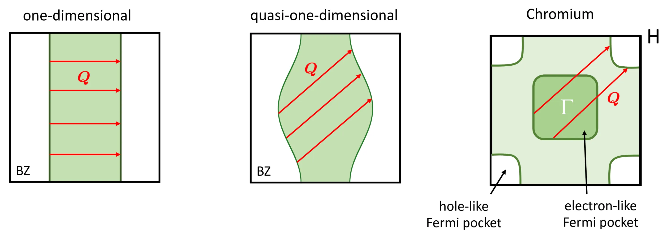
\begin{array}{r} ρ (r) = ρ_{0} + δ ρ \cos (Q \cdot r), \end{array}

with $δ ρ ≪ ρ_{0}$ . The spin density states frequently appear in low-dimensional systems like organic conductors, or in transition metals such as chromium (Cr) for example. In all cases, nesting plays an important role:

Attachments/Script 74.webp|700

In quasi-one-dimensional electron systems, a main direction of motion dominates over two other directions with weak dispersion. In this case, the nesting condition is very probable to be fulfilled, as it is schematically shown in the centre panel of the figure above. Chromium is a three-dimensional metal, where nesting occurs between an electron-like Fermi surface around the $Γ$ -point and a hole-like Fermi surface at the Brillouin zone boundary ( $H$ -point). These Fermi surfaces originate in different bands (right panel in the figure shown above). Chromium has a body-centred cubic crystal structure, where the $H$ -point at $(π / a, 0, 0)$ leads to the nesting vector $Q_{x} ∥ (1, 0, 0)$ and equivalent vectors in $y$ - and $z$ -direction, which are incommensurable with the lattice.

The textbook example of nesting is found in a tight-binding model of a simple cubic lattice with nearest-neighbour hopping at half filling. The band structure is given by

\begin{array}{r} ϵ_{k} = - 2 t [\cos (k_{x} a) + \cos (k_{y} a) + \cos (k_{z} a)], \end{array}

where $a$ is the lattice constant and $t$ the hopping term. Because of half filling, the chemical potential $μ = ϵ_{F}$ lies at $μ = 0$ such that $ξ_{k} = ϵ_{k}$ . Obviously, $ϵ_{k + Q} = - ϵ_{k}$ holds for all $k$ , for the nesting vector $Q = (π / a) (1, 1, 1)$ . This full nesting trait is a signature of the total particle-hole symmetry, meaning in the ground state there are as many occupied as empty states. Analogously to the Peierls instability, the spin density wave induces the opening of a gap at the Fermi surface. This is another example of a Fermi surface instability. In this situation, the gap is confined to the areas of the Fermi surface obeying the nesting condition. Contrary to the ferromagnetic order, the material can become insulating when forming the spin density wave state.

7.3 Stoner Excitations

In this last section, we discuss the elementary excitations of the ferromagnetic ground state with $n_{↑} > n_{↓}$ , including both particle-hole excitations and collective modes. For this purpose we use the Stoner model Hamiltonian, introduced earlier, which we write here entirely in momentum space operators,

\begin{array}{r} H = \sum_{k, s} ϵ_{k} {\hat{c}}_{k s}^{†} {\hat{c}}_{k s} + \frac{U}{Ω} \sum_{k, k^{'}, q^{'}} {\hat{c}}_{k + q^{'} ↑}^{†} {\hat{c}}_{k ↑} {\hat{c}}_{k^{'} - q^{'} ↓}^{†} {\hat{c}}_{k^{'} ↓} . \end{array}

The spin polarised ground state $| ψ_{g} ⟩$ can be written on the mean field level as

\begin{array}{r} | ψ_{g} ⟩ = \prod_{| k | \leq k_{F ↓}} {\hat{c}}_{k ↓}^{†} \prod_{| k | \leq k_{F ↑}} {\hat{c}}_{k ↑}^{†} | o ⟩ \end{array}

with $k_{F s} = {(6 π^{2} n_{s})}^{1 / 3}$ .
We now consider spin excitations, for which we make the Ansatz

\begin{array}{r} | ψ_{q} ⟩ = \sum_{k} f_{k} {\hat{c}}_{k + q ↓}^{†} {\hat{c}}_{k ↑} | ψ_{g} ⟩ = \sum_{k} f_{k} | ψ_{k, q} ⟩ . \end{array}

This is a superposition of states where a spin up electron is removed from the ground state $| ψ_{g} ⟩$ and placed back with opposite spin and a fixed momentum transfer $q$ . The simple electron-hole excitation with such a spin flip corresponds to the state $| ψ_{k, q} ⟩ = {\hat{c}}_{k + q ↓}^{†} {\hat{c}}_{k ↑} | ψ_{g} ⟩$ and has the energy

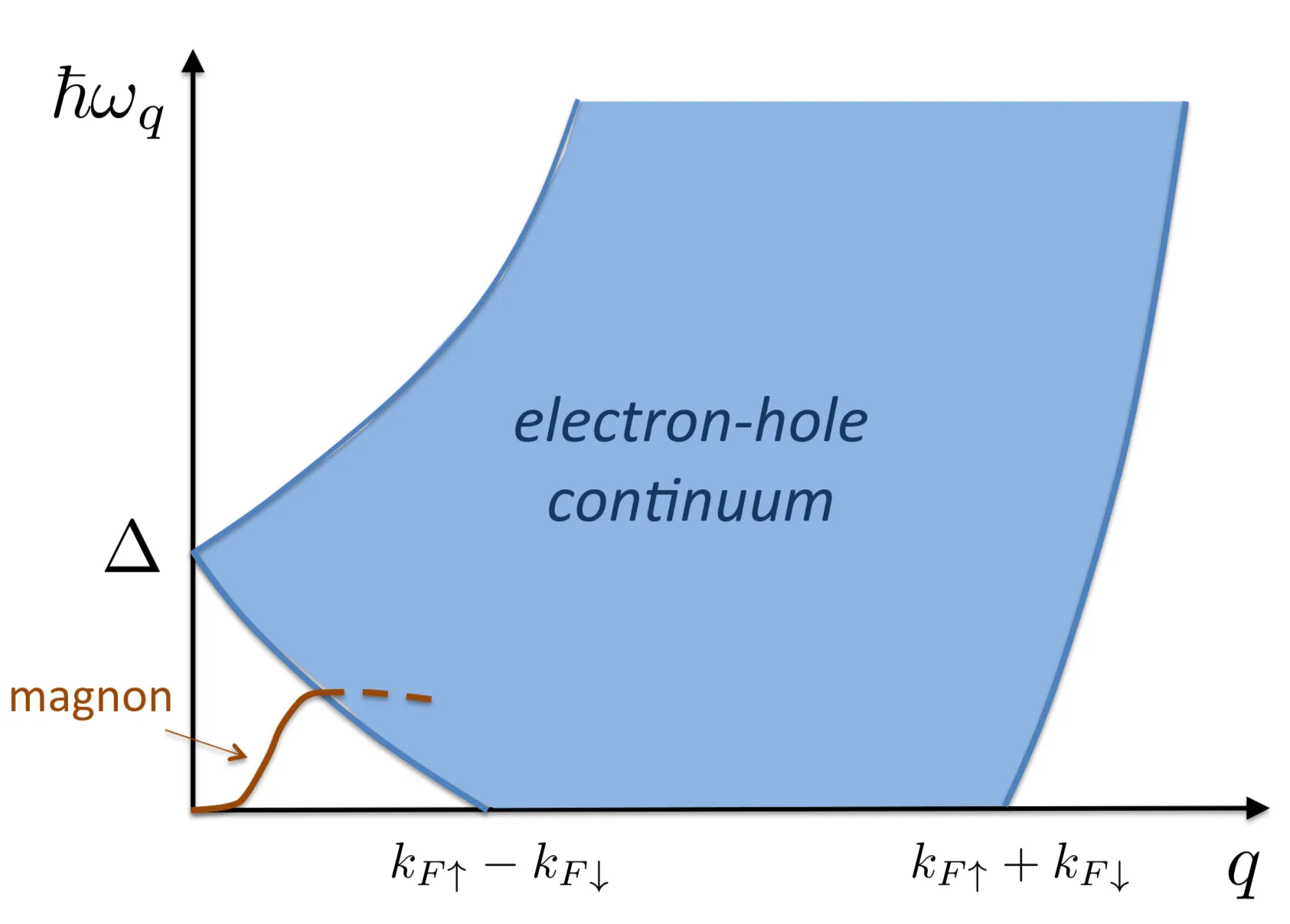
\begin{array}{r} E_{k, q} = ϵ_{k + q ↓} - ϵ_{k ↑} = ϵ_{k + q} - ϵ_{k} + U (n_{↑} - n_{↓}) = ϵ_{k + q} - ϵ_{k} + Δ . \end{array}

We have to ensure that an electron with $(k, ↑)$ is available to be removed, and that the state $(k + q, ↓)$ is unoccupied. The independent electron-hole part of the spectrum constitutes a continuum of excitations and is depicted by the shaded region:

Attachments/Script 75.webp|700

Note that the spin splitting of the spectrum opens a window in the low-energy low-momentum transfer sector of the excitations.
The excitation energy of $| ψ_{q} ⟩$ can be obtained by solving the following Schrödinger equation

\begin{array}{r} H | ψ_{q} ⟩ = (E_{g} + ℏ ω_{q}) | ψ_{q} ⟩, \end{array}

with $E_{g}$ as the ground state energy $(H | ψ_{g} ⟩ = E_{g} | ψ_{g} ⟩)$ . Actually it is more convenient to rearrange this equation into the following form to eliminate $E_{g}$ ,

\begin{array}{r} ℏ ω_{q} | ψ_{q} ⟩ = \sum_{k} f_{k} [H, {\hat{c}}_{k + q ↓}^{†} {\hat{c}}_{k ↑}] | ψ_{g} ⟩ . \end{array}

Evaluating the commutator we obtain

\begin{array}{r} \begin{aligned} ℏ ω_{q} | ψ_{q} ⟩ = (ϵ_{k + q} - & ϵ_{k}) | ψ_{q} ⟩ \\ + & \frac{U}{Ω} \sum_{k} f_{k} \sum_{k^{'}, q^{'}} {{\hat{c}}_{k^{'} + q^{'} ↑}^{†} {\hat{c}}_{k^{'} ↑} {\hat{c}}_{k + q - q^{'} ↓}^{†} {\hat{c}}_{k ↑} - {\hat{c}}_{k + q ↓}^{†} {\hat{c}}_{k - q^{'} ↑} {\hat{c}}_{k^{'} - q^{'} ↓}^{†} {\hat{c}}_{k^{'} ↓}} | ψ_{g} ⟩ . \end{aligned} \end{array}

The terms with four $\hat{c}$ -operators are not so easy to handle. Therefore we adopt a mean field point of view in the analogous way as before and decouple these terms through the following approximation,

\begin{array}{r} \begin{aligned} {\hat{c}}_{k^{'} + q^{'} ↑}^{†} {\hat{c}}_{k^{'} ↑} {\hat{c}}_{k + q - q^{'} ↓}^{†} {\hat{c}}_{k ↑} - {\hat{c}}_{k + q ↓}^{†} {\hat{c}}_{k - q^{'} ↑} {\hat{c}}_{k^{'} - q^{'} ↓}^{†} {\hat{c}}_{k^{'} ↓} \\ ⟶ δ_{q^{'}, 0} (n_{k^{'} ↑} - n_{k^{'} ↓}) {\hat{c}}_{k + q, ↓}^{†} {\hat{c}}_{k ↑} + (n_{k + q ↓} δ_{k^{'}, k + q} - n_{k ↑} δ_{k, k^{'} + q^{'}}) {\hat{c}}_{k - q^{'} + q ↓}^{†} {\hat{c}}_{k - q^{'} ↑} \end{aligned} \end{array}

The basic scheme is to combine $\hat{c}$ -operators in the four-operator expression so as to obtain a density-operator-like expression ${\hat{c}}_{k s}^{†} {\hat{c}}_{k s}$ (this introduces some constraints on the momenta implemented) which then is replaced by its mean value $n_{k s}$ . In this process it turns out that the remaining two operators combine to ${\hat{c}}_{k + q ↓}^{†} {\hat{c}}_{k ↑}$ -like factors to construct $| ψ_{q} ⟩$ . This helps then to "close" the Schrödinger equation for the wave function $f_{k}$ . We replace $n_{k s}$ with the Fermi-Dirac distribution for electrons of spin $s$ with the energy $ϵ_{k s}$ .
We insert this approximation into the Schrödinger equation (written above) and multiply from the left with $⟨ ψ_{\tilde{k}, q} | = ⟨ ψ_{g} | {\hat{c}}_{\tilde{k} ↑} {\hat{c}}_{\tilde{k} + q ↓}^{†}$ to obtain the projected equation,

\begin{array}{r} f_{\tilde{k}} {ℏ ω_{q} - ϵ_{\tilde{k} + q} + ϵ_{\tilde{k}} - U (n_{↑} - n_{↓})} = \frac{U}{Ω} \sum_{k} f_{k} (n_{k + q ↓} - n_{k ↑}) = R_{q} \end{array}

where we used that the density of electrons of spin $s$ is given by

\begin{array}{r} n_{s} = \frac{1}{Ω} \sum_{k^{'}} n_{k^{'} s} . \end{array}

and we defined $R_{q}$ . We solve now the equation for the wave function $f_{k}$ and obtain

\begin{array}{r} f_{k} = \frac{R_{q}}{ℏ ω_{q} - ϵ_{k + q ↓} + ϵ_{k ↑}} \end{array}

with $ϵ_{k s} = ϵ_{k} + U n_{\bar{s}}$ . We use now $f_{k}$ to re-express $R_{q}$ which yields the equation,

\begin{array}{r} R_{q} = U R_{q} \frac{1}{Ω} \sum_{k} \frac{n_{k + q ↓} - n_{k ↑}}{ℏ ω_{q} - ϵ_{k + q ↓} + ϵ_{k ↑}} \end{array}

which can be used to determine $ℏ ω_{q}$ for $R_{q} \neq 0$ . The solutions contain, in principle, also the continuum of the electron-hole excitations discussed above. We focus, however, now on the non-trivial collective mode. It is easy to see that in the $q \to 0$ limit we find

\begin{array}{r} 1 = \frac{U (n_{↓} - n_{↑})}{ℏ ω_{0} - U (n_{↑} - n_{↓})} \Rightarrow ℏ ω_{0} = 0 \end{array}

indicating that there are excitations for small $q$ . Note that for $q = 0$ we find $f_{k} =$ const. independent of $k$ which we will use later.
We calculate now the dispersion for small $q (≪ k_{F})$ . For the concrete calculation we will assume that $ϵ_{k} = ℏ^{2} k^{2} / 2 m$ to obtain analytical results. Using the fact that $ℏ ω_{q} ≪ Δ$ we can expand the equation leading to

\begin{array}{r} ℏ ω_{q} \approx [1 + \frac{U}{Ω} \sum_{k} \frac{n_{k + q ↓} - n_{k ↑}}{ϵ_{k + q ↓} - ϵ_{k ↑}}] {[- \frac{U}{Ω} \sum_{k} \frac{n_{k + q ↓} - n_{k ↑}}{{(ϵ_{k + q ↓} - ϵ_{k ↑})}^{2}}]}^{- 1} . \end{array}

For small $q$ we expand up to order $q^{2}$ (actually $q$ -linear contributions cancel),

\begin{array}{r} \begin{aligned} \frac{U}{Ω} \sum_{k} \frac{n_{k + q ↓} - n_{k ↑}}{ϵ_{k + q} - ϵ_{k} + Δ} & \approx \frac{U}{Ω} \sum_{k} \frac{n_{k + q ↓} - n_{k ↑}}{Δ} {1 - \frac{ϵ_{k + q} - ϵ_{k}}{Δ} + {(\frac{ϵ_{k + q} - ϵ_{k}}{Δ})}^{2}} \\ \approx - 1 + \frac{U}{Ω} \sum_{k} {\frac{n_{k ↑} + n_{k ↓}}{Δ^{2}} \frac{ℏ^{2} q^{2}}{2 m} - \frac{n_{k ↑} - n_{k ↓}}{Δ^{2}} \frac{{(2 ℏ^{2} k \cdot q)}^{2}}{4 m^{2} Δ}} \\ \approx - 1 + \frac{ℏ^{2} q^{2}}{2 m Δ^{2}} (U n_{0} - \frac{4 ϵ_{F}}{3}) \end{aligned} \end{array}

and analogously

\begin{array}{r} \frac{U}{Ω} \sum_{k} \frac{n_{k + q ↓} - n_{k ↑}}{{(ϵ_{k + q} - ϵ_{k} + Δ)}^{2}} \approx - \frac{1}{Δ} \end{array}

such that we obtain

\begin{array}{r} ℏ ω_{q} \approx \frac{ℏ^{2} q^{2}}{2 m Δ} \frac{2 ϵ_{F}}{3} (U N (ϵ_{F}) - 2) \sim \frac{ℏ^{2} q^{2}}{2 m} {(\frac{U}{U_{c}} - 1)}^{1 / 2} . \end{array}

Where we use that $Δ \sim {(U - U_{c})}^{1 / 2}$ for $U \to U_{c}$ . Hence, if $U > U_{c} = 2 / N (ϵ_{F})$ we find $ℏ ω_{q} > 0$ . Since the elementary excitations have an energy gap of the order of $Δ$ at small $q$ , the collective excitations, which are termed magnons, are well-defined quasiparticles describing propagating spin waves. When these modes enter the electron-hole continuum, they are damped in the same way as plasmons decay into the electron-hole continuum.

Being a bound state composed of an electron and a hole, magnons are bosonic quasiparticles. This collective excitation features a $q^{2}$ -dependent dispersion with a vanishing excitation energy in the limit $q \to 0$ . This property represents a case of the so-called Goldstone theorem which states that there is a gapless $q = 0$ excitation in every ordered phase which originates from the spontaneous breaking of a continuous symmetry. Remark: It is important that the symmetry is broken spontaneously and not by an external field, because we need a continuous set of ground states, here through spin rotation. With an external field we would have only one ground state and all other orientations of the magnetisation would have higher energy. Then the $q = 0$ mode would have a finite energy. In our case the continuous symmetry is spin rotation and the ferromagnetic state breaks this symmetry by choosing spontaneously the direction of magnetisation. We defined this direction as the $z$ -axis such that the total spin $z$ -component is $S_{tot}^{z} = \frac{1}{2} (N_{↑} - N_{↓})$ . Any of the $2 S_{tot} + 1$ degenerate ground states can be reached by continued application of the spin lowering operator ${\hat{S}}_{tot}^{-}$ which lowers $S_{tot}^{z}$ by 1,

\begin{array}{r} \begin{array}{l} {\hat{S}}_{tot}^{z} | ψ_{g} ⟩ = ℏ S_{tot}^{z} | ψ_{g} ⟩ \\ {\hat{S}}_{tot}^{2} | ψ_{g} ⟩ = ℏ^{2} S_{tot} (S_{tot} + 1) | ψ_{g} ⟩ \end{array}} \Rightarrow {\begin{cases} [{\hat{S}}_{tot}^{2}, {\hat{S}}_{tot}^{-}] = 0, | ψ_{g}^{'} ⟩ = {\hat{S}}_{tot}^{-} | ψ_{g} ⟩ \\ {\hat{S}}_{tot}^{2} | ψ_{g}^{'} ⟩ = ℏ^{2} S_{tot} (S_{tot} + 1) | ψ_{g}^{'} ⟩ \end{cases} \end{array}

The spin lowering operator can be written as

\begin{array}{r} {\hat{S}}_{tot}^{-} = \frac{ℏ}{Ω} \sum_{k} {\hat{c}}_{k ↓}^{†} {\hat{c}}_{k ↑} \end{array}

which notably is the operator generating $| ψ_{q = 0} ⟩$ , where, as mentioned, $f_{k} = 1 / Ω$ is independent of $k$ . From the equation before, we understand that $| ψ_{q = 0} ⟩$ is simply another ground state $| ψ_{g}^{'} ⟩$ and has, thus, the same energy as $| ψ_{g} ⟩$ . We conclude, therefore, that $ℏ ω_{q = 0} = 0$ .

7 Magnetism in Metals

7.1 Stoner Instability

7.1.1 Stoner Model Within the Mean Field Approximation

7.1.2 Stoner Criterion

7.1.3 Spin Susceptibility for T>TC

7.2 General Spin Susceptibility and Magnetic Instabilities

7.2.1 General Dynamic Spin Susceptibility

7.2.2 Instability with Finite Wave Vector Q

7.2.3 Influence of the Band Structure

7.3 Stoner Excitations

7.1.3 Spin Susceptibility for $T > T_{C}$

7.2.2 Instability with Finite Wave Vector $Q$