Jump back to chapter selection.

Table of Contents

6.1 Electrical Conductivity
6.2 Transport Equations and Relaxation Time
6.3 Impurity Scattering
6.4 Electron-Phonon Scattering
6.5 Electron-Electron Scattering
6.6 Matthiessen's Rule and the Ioffe-Regel Limit
6.7 General Transport Coefficients
6.8 Anderson Localisation in One-Dimensional Systems

6 Transport Properties of Metals

The ability to transport electrical current is one of the most remarkable and characteristic properties of metals. At zero temperature, an ideal pure metal is a perfect electrical conductor, that is, its resistivity is zero. However, disorder due to impurities and lattice defects influence the transport and yield a finite residual resistivity, as found in real materials. At finite temperature, electron-electron and electron-phonon scattering lead to a temperature-dependent resistivity. Furthermore, an external magnetic field may influence the resistivity, a phenomenon called magnetoresistance, and also leads to the previously studied Hall effect. In this chapter, the effects of a magnetic field will not be considered. Finally, heat transport, which is also mostly mediated by electrons in metals, goes hand in hand with the electric transport. In this context, transport phenomena such as thermoelectricity (Seebeck and Peltier effect) will be analysed here.

6.1 Electrical Conductivity

In a normal metal, an electrical current density $j (q, ω)$ (in $q, ω$ -space) is induced by an applied electrical field $E (q, ω)$ . For a homogeneous isotropic metal, we define the scalar (note that in an anisotropic material, the conductivity $\hat{σ}$ would be a full $3 \times 3$ tensor) electrical conductivity $σ (q, ω)$ within linear response, through

\begin{array}{r} j (q, ω) = σ (q, ω) E (q, ω) . \end{array}

The current density $j (q, ω)$ is related to the charge density $ρ (r, t) = - e n (r, t)$ , via the continuity equation

\begin{array}{r} \frac{\partial}{\partial t} ρ (r, t) + \nabla \cdot j (r, t) = 0 \end{array}

or, in Fourier transformed,

\begin{array}{r} ω ρ (q, ω) - q \cdot j (q, ω) = 0. \end{array}

It is interesting to see that a relation between the conductivity $σ (q, ω)$ and the dynamical dielectric susceptibility $χ_{0} (q, ω)$ defined in Chapter 3 arises from the definition of conductivity and the continuity equation. For this, we can calculate

\begin{aligned} χ_{0} (q, ω) & = - \frac{ρ (q, ω)}{e V (q, ω)} = - \frac{q \cdot j (q, ω)}{e ω V (q, ω)} \\ = - \frac{σ (q, ω)}{ω e} \frac{q \cdot E (q, ω)}{V (q, ω)} = - \frac{σ (q, ω)}{ω e} \frac{i | q |^{2} V (q, ω)}{e V (q, ω)} . \end{aligned}

In the first line, we used the definition of $χ_{0} (q, ω)$ and the continuity equation. To the second line, we made use of the definition of $σ (q, ω)$ and then replaced $E (q, ω)$ by $i q V (q, ω) / e$ , which is nothing else than the Fourier transform of the equation

\begin{array}{r} - e E (r, t) = - \nabla_{r} V (r, t) . \end{array}

From these calculations we conclude that

\begin{array}{r} χ_{0} (q, ω) = \frac{- i | q |^{2}}{e^{2} ω} σ (q, ω), \end{array}

and thus

\begin{array}{r} ε (q, ω) = 1 - \frac{4 π e^{2}}{| q |^{2}} χ_{0} (q, ω) = 1 + \frac{4 π i}{ω} σ (q, ω) . \end{array}

In the limit of large wavelengths $| q | ≪ k_{F}$ , we know from previous discussions that $ε (0, ω) = 1 - ω_{p}^{2} / ω^{2}$ . Then the conductivity simplifies to

\begin{array}{r} σ (ω) = \frac{i ω_{p}^{2}}{4 π ω} . \end{array}

One might conclude from this result that the conductivity is purely imaginary in the small- $| q |$ limit. However, this conclusion is wrong, since the real part of $σ (ω)$ is related to its imaginary part via the Kramers-Kronig relation. Defining $σ_{1} (σ_{2})$ as the real (imaginary) part of $σ$ , this relation states that

\begin{array}{r} σ_{1} (ω) = - \frac{1}{π} P [\int_{- \infty}^{+ \infty} d ω^{'} \frac{1}{ω - ω^{'}} σ_{2} (ω^{'})] \end{array}

and

\begin{array}{r} σ_{2} (ω) = \frac{1}{π} P [\int_{- \infty}^{+ \infty} d ω^{'} \frac{1}{ω - ω^{'}} σ_{1} (ω^{'})] . \end{array}

A simple calculation with the expression for $σ_{2} (ω)$ from the ideal conductor, yields

\begin{aligned} σ_{1} (ω) & = \frac{ω_{p}^{2}}{4} δ (ω) \\ σ_{2} (ω) & = \frac{ω_{p}^{2}}{4 π ω} . \end{aligned}

Obviously this metal is perfectly conducting ( $σ \to \infty$ for $ω \to 0$ ), which comes from the fact that we considered systems without dissipation so far. An additional important property coming from complex analysis, is the existence of the so-called f-sum rule,

\begin{array}{r} \int_{0}^{\infty} d ω^{'} σ_{1} (ω^{'}) = \frac{1}{2} \int_{- \infty}^{+ \infty} d ω^{'} σ_{1} (ω^{'}) = \frac{ω_{p}^{2}}{8} = \frac{π e^{2} n}{2 m} . \end{array}

This relation is valid for all electronic systems (including semiconductors).

6.2 Transport Equations and Relaxation Time

We introduce here Boltzmann's transport theory as a rather simple and efficient way to deal with dissipation and momentum relaxation of non-stationary electronic states in metals.

6.2.1 The Boltzmann Equation

In order to tackle the problem of a finite conductivity, we use a formalism similar to Landau's Fermi liquid theory, based on a distribution function of quasi-particles. In transport theory, the distribution function can be used to describe the deviation of the system from an equilibrium. If the system is isolated from external influence, equilibrium is reached through relaxation after some time, a process which is accompanied with an increase of entropy as discussed in statistical physics. Analogously to the theory of transport phenomena, let us introduce the distribution function $f (k, r, t)$ , where

\begin{array}{r} f (k, r, t) \frac{d^{3} k}{(2 π)^{3}} d^{3} r \end{array}

is the number of particles in the infinitesimal phase space volume $d^{3} r d^{3} k / (2 π)^{3}$ centred at $(k, r)$ , at time $t$ . Note that, for simplicity, we neglect the electron spin. In general there would be a distribution function for each spin species. Such a description is only applicable if the temporal and spacial variations occur at long wavelengths and small frequencies, respectively, that is, if typically $| q | ≪ k_{F}$ and $ℏ ω ≪ ϵ_{F}$ . The total number of particles $N$ is given by

\begin{array}{r} N = 2 \int \frac{d^{3} k}{(2 π)^{3}} d^{3} r f (k, r, t) . \end{array}

The equilibrium distribution $f_{0}$ for the Fermionic quasi-particles is given by the Fermi-Dirac distribution,

\begin{array}{r} f_{0} (k, r, t) = \frac{1}{e^{(ϵ_{k} - μ) / k_{B} T} + 1}, \end{array}

and is independent of space $r$ and time $t$ . The general distribution function $f (k, r, t)$ obeys the Boltzmann equation

\begin{array}{r} \frac{D}{D t} f (k, r, t) = (\frac{\partial}{\partial t} + \dot{r} \cdot \nabla_{r} + \dot{k} \cdot \nabla_{k}) f (k, r, t) = {(\frac{\partial f}{\partial t})}_{coll} \end{array}

where the substantial derivative in phase space $D / D t$ is defined as the total temporal derivative in a frame moving with the phase-space volume. The right-hand side is called collision integral and describes the rate of change in $f$ due to collision processes. Without scattering, this equation would represent a continuity equation for $f$ . Now, consider the temporal derivatives of $r$ and $k$ from a quasi-classical viewpoint. In absence of a magnetic field, we find

\begin{aligned} \dot{r} & = \frac{ℏ k}{m} \\ ℏ \dot{k} & = - e E \end{aligned}

that is, the force $ℏ \dot{k}$ , which is our central interest, originates from the electric field. The collision integral may be expressed via the probability $W (k, k^{'})$ to scatter a quasi-particle with wave vector $k$ to $k^{'}$ . For simple scattering on static potentials, the collision integral is given by

\begin{aligned} {(\frac{\partial f}{\partial t})}_{coll} = - \int \frac{d^{3} k^{'}}{(2 π)^{3}} & [W (k, k^{'}) f (k, r, t) (1 - f (k^{'}, r, t)) \\ - W (k^{'}, k) f (k^{'}, r, t) (1 - f (k, r, t))] . \end{aligned}

The first term, describing the scattering from $k$ to $k^{'}$ , requires a quasi-particle at $k$ , hence the factor $f (k, r, t)$ , and the absence of a particle at $k^{'}$ , therefore the factor $1 - f (k^{'}, r, t)$ . Note that if spin was considered here, this collision term would account for scattering processes where spin is conserved. However, there are in principle also scattering process where the electron spin can be transferred to the lattice (spin-orbit coupling) or an impurity (Kondo effect) and would not be conserved independently. This process describes the scattering out of the phase space volume $d^{3} k / (2 π)^{3}$ , that is, reduces the number of particles in it. Therefore, it enters the collision integral with negative sign. The second term describes the opposite process and, according to its positive sign, increases the number of particles in the phase space volume $d^{3} k / (2 π)^{3}$ . For a system with time inversion symmetry, we have $W (k, k^{'}) = W (k^{'}, k)$ . Assuming this, we can combine both terms and end up with

\begin{array}{r} {(\frac{\partial f}{\partial t})}_{coll} = \int \frac{d^{3} k^{'}}{(2 π)^{3}} W (k, k^{'}) [f (k^{'}, r, t) - f (k, r, t)] . \end{array}

The Boltzmann equation is a complicated integro-differential equation and suitable approximations are required. Usually, we study processes close to equilibrium, where the deviation $f (k, r, t) - f_{0} (k, r, t)$ is small compared to $f (k, r, t)$ . Here, to generalise we assume $f_{0} (k, r, t)$ to be a local equilibrium distribution for which the temperature $T = T (r, t)$ and the chemical potential $μ = μ (r, t)$ vary slowly in $r$ and $t$ , such that $f_{0} (k, r, t)$ can still be expressed via the local Fermi-Dirac distribution. At small deviations from equilibrium (or local equilibrium), we can approximate the collision integral by the relaxation-time approximation. For simplicity, we assume that the system is isotropic, such that the quasi-particle dispersion $ϵ_{k}$ only depends on $| k |$ and, furthermore, that the scattering probabilities are elastic and depend on the angle between $k$ and $k^{'}$ . Then, we make the Ansatz

\begin{array}{r} {(\frac{\partial f}{\partial t})}_{coll} = - \frac{f (k, r, t) - f_{0} (k, r, t)}{τ (ϵ_{k})} . \end{array}

The time scale $τ (ϵ_{k})$ is called relaxation time and gives the characteristic time within which the system relaxes to equilibrium.

Consider the simplest case of a system at constant temperature subject to a small uniform electric field $E (t)$ . With $f (k, r, t) = f_{0} (k, r, t) + δ f (k, r, t)$ , we can calculate the Fourier-transform of Boltzmann equation in relaxation-time approximation and find, after linearising in $δ f$ ,

\begin{array}{r} - i ω δ f (k, ω) - \frac{e E (ω)}{ℏ} \nabla_{k} f_{0} (k) = - \frac{δ f (k, ω)}{τ (ϵ_{k})} \end{array}

with

\begin{array}{r} f (k, t) = \int_{- \infty}^{+ \infty} \frac{d ω}{2 π} f (k, ω) e^{- i ω t} \end{array}

and

\begin{array}{r} E (t) = \int_{- \infty}^{+ \infty} \frac{d ω}{2 π} E (ω) e^{- i ω t} . \end{array}

In order to come to this expression, we used that $f (k, r, t) = f (k, t)$ for $E = E (t)$ are spacially uniform, and assumed for linearising that $δ f \sim | E |$ . Thus, this equation is consistent to linear order in $| E |$ and can be easily solved as

\begin{array}{r} δ f (k, ω) = \frac{e τ (ϵ_{k}) E (ω)}{ℏ (1 - i ω τ (ϵ_{k}))} \nabla_{k} f_{0} (k) = \frac{e τ (ϵ_{k}) E (ω)}{ℏ (1 - i ω τ (ϵ_{k}))} \frac{\partial f_{0} (ϵ_{k})}{\partial ϵ_{k}} \nabla_{k} ϵ_{k} . \end{array}

This result leads straightforwardly to the quasi-particle current $j (ω)$ ,

\begin{aligned} j (ω) & = - 2 e \int \frac{d^{3} k}{(2 π)^{3}} v_{k} f (k, ω) \\ = - \frac{e^{2}}{4 π^{3}} \int d^{3} k \frac{τ (ϵ_{k}) [E (ω) \cdot v_{k}] v_{k}}{1 - i ω τ (ϵ_{k})} \frac{\partial f_{0} (ϵ_{k})}{\partial ϵ_{k}} \end{aligned}

with $ℏ v_{k} = \nabla_{k} ϵ_{k}$ , which in turn can be simplified to

\begin{array}{r} j_{α} (ω) = \sum_{β} σ_{α β} (ω) E_{β} (ω), \end{array}

where the conductivity tensor $σ_{α β}$ reads

\begin{array}{r} σ_{α β} = - \frac{e^{2}}{4 π^{3}} \int d ϵ \frac{\partial f_{0} (ϵ)}{\partial ϵ} \frac{τ (ϵ)}{1 - i ω τ (ϵ)} \int d Ω_{k} | k |^{2} \frac{v_{α k} v_{β k}}{ℏ | v_{k} |} . \end{array}

This corresponds to the Ohmic law. Note that $σ_{α β} = σ δ_{α β}$ in isotropic systems. We recover in this case the expression for the conductivity, which we introduced at the beginning of this chapter. It is also important to notice that $\partial f_{0} (ϵ) / \partial ϵ$ concentrates around $ϵ = μ$ for $T ≪ T_{F}$ . In the following, we consider this result for an isotropic system in different limiting cases.

6.2.2 The Drude Form

For $ω τ ≫ 1$ the expression for $σ_{α β}$ becomes independent on the relaxation time. In an isotropic system $σ_{α β} = σ δ_{α β}$ at low temperatures $T ≪ T_{F}$ , this leads to

\begin{array}{r} σ (ω) \approx i \frac{e^{2} m^{2} v_{F}}{4 π^{3} ℏ^{3} ω} \int d Ω_{k} v_{F x}^{2} = i \frac{e^{2} n}{m ω} = i \frac{ω_{p}^{2}}{4 π ω}, \end{array}

which reproduces the previous result for ideal conductors. However now, this does not mean that our system is a perfect conductor, as becomes clear when we turn towards small $ω (ω τ ≪ 1)$ . We are actually interested in the static limit, where the "dc conductivity" ( $ω = 0$ ; "dc" means "direct current") reduces to

\begin{array}{r} σ = - \frac{e^{2} n}{m} \int d ϵ \frac{\partial f_{0}}{\partial ϵ} τ (ϵ) = \frac{e^{2} n \bar{τ}}{m} = \frac{ω_{p}^{2} \bar{τ}}{4 π} . \end{array}

Since the function $\partial f_{0} / \partial ϵ$ is strongly peaked around the Fermi energy $ϵ_{F}$ , we introduced a mean relaxation time $\bar{τ} = - \int d ϵ τ (ϵ) \partial f_{0} / \partial ϵ$ . This form recovers the well-known Drude form of the conductivity. Note, that the phenomenological Drude theory of electron transport can be deduced from purely classical considerations.

If the relaxation time $τ$ depends only weakly on energy, we can simply calculate the optical conductivity at finite frequency,

\begin{aligned} σ (ω) & = \frac{ω_{p}^{2}}{4 π} \frac{\bar{τ}}{1 - i ω \bar{τ}} = \frac{ω_{p}^{2}}{4 π} (\frac{\bar{τ}}{1 + ω^{2} {\bar{τ}}^{2}} + i \frac{{\bar{τ}}^{2} ω}{1 + ω^{2} {\bar{τ}}^{2}}) \\ = σ_{1} + i σ_{2} . \end{aligned}

Note that the real part satisfies the $f$ -sum rule,

\begin{array}{r} \int_{0}^{\infty} d ω σ_{1} (ω) = \int_{0}^{\infty} d ω \frac{ω_{p}^{2}}{4 π} \frac{\bar{τ}}{1 + ω^{2} {\bar{τ}}^{2}} = \frac{ω_{p}^{2}}{8} \end{array}

and that $σ (ω)$ recovers the behaviour of $σ_{1} (ω)$ in dissipationless systems in the limit $\bar{τ} \to \infty$ . Note that $σ_{1} (ω)$ has Lorentzian form and naturally leads to a delta function:

\begin{array}{r} σ_{1} (ω) = \frac{ω_{p}^{2}}{4 π} \frac{\bar{τ}}{1 + ω^{2} {\bar{τ}}^{2}} \overset{\bar{τ} \to \infty}{\to} \frac{ω_{p}^{2}}{4} δ (ω) . \end{array}

This form of the conductivity yields the dielectric function

\begin{array}{r} ε (ω) = 1 - \frac{ω_{p}^{2} \bar{τ}}{ω (i + ω \bar{τ})} = 1 - \frac{ω_{p}^{2} {\bar{τ}}^{2}}{1 + ω^{2} {\bar{τ}}^{2}} + i \frac{1}{ω} \frac{ω_{p}^{2} \bar{τ}}{1 + ω^{2} {\bar{τ}}^{2}} \end{array}

which can be used to discuss the optical properties of metals. The complex index of refraction $n + i κ$ is given through $(n + i κ)^{2} = ε$ . Next, we discuss three important regimes of frequency. To probe optical properties we consider the reflectivity of light hitting a metal surface perpendicularly. Then the reflectivity is given by

\begin{array}{r} R = \frac{(n - 1)^{2} + κ^{2}}{(n + 1)^{2} + κ^{2}} . \end{array}

Inside the metal the light propagation is renormalised by $k \to k (n + i κ)$ with $k = ω / c$ such that

\begin{array}{r} e^{i k (n + i κ) z} = e^{i k n z} e^{- κ k z} = e^{i k n z} e^{- z / δ} \end{array}

defining the penetration length

\begin{array}{r} δ = \frac{c}{ω κ} . \end{array}

Relaxation-free regime $(ω \bar{τ} ≪ 1 ≪ ω_{p} \bar{τ})$

In this limit, the real $(ε_{1})$ and imaginary $(ε_{2})$ part of the dielectric function read

\begin{aligned} ε_{1} (ω) & \approx - ω_{p}^{2} {\bar{τ}}^{2} \\ ε_{2} (ω) & \approx \frac{ω_{p}^{2} \bar{τ}}{ω} . \end{aligned}

The real part $ε_{1}$ is constant and negative, whereas the imaginary part $ε_{2}$ becomes singular in the limit $ω \to 0$ . Thus, the refractive index turns out to be dominated by $ε_{2}$

\begin{array}{r} n (ω) \approx κ (ω) \approx \sqrt{\frac{ε_{2} (ω)}{2}} \approx \sqrt{\frac{ω_{p}^{2} \bar{τ}}{2 ω}} ≫ 1. \end{array}

As a result, the reflectivity $R$ is practically $100 %$ . The absorption index $κ (ω)$ determines the penetration depth $δ$ through

\begin{array}{r} δ (ω) = \frac{c}{ω κ (ω)} \approx \frac{c}{ω_{p}} \sqrt{\frac{2}{ω \bar{τ}}} . \end{array}

With this, the skin depth of a metal with the famous relation $δ (ω) \sim ω^{- 1 / 2}$ is reproduced within the relaxation time approximation of the Boltzmann equation. While length $δ (ω)$ is in the centimetre range for frequencies of the order of $10 - 100 Hz$ , the Debye length $c / ω_{p}$ , is only of the order of $100 Å$ for $ℏ ω_{p} = 10 eV$ .

Relaxation regime ( $1 ≪ ω \bar{τ} ≪ ω_{p} \bar{τ}$ )

Here, we can expand the dielectric function in $(ω \bar{τ})^{- 1}$ , yielding

\begin{array}{r} ε (ω) = 1 - \frac{ω_{p}^{2}}{ω^{2}} + i \frac{ω_{p}^{2}}{ω^{3} \bar{τ}} . \end{array}

The real part $ε_{1} \approx - ω_{p}^{2} / ω^{2}$ is large and negative and dominates in magnitude over $ε_{2}$ . For the optical properties, we obtain

\begin{aligned} κ (ω) & \approx \frac{ω_{p}}{ω} \\ n (ω) & \approx \frac{ω_{p}}{2 ω^{2} \bar{τ}} . \end{aligned}

We find $κ (ω) ≫ n (ω) ≫ 1$ , which implies a large reflectivity of metals in this frequency range as well. Note that visible frequencies are part of this regime:

Attachments/Script 59.webp|700
Attachments/Script 60.webp|700

The frequency dependence of the penetration depth becomes weak, and its magnitude is approximately given by the Debye length, $δ \sim c / ω_{p}$ .

Ultraviolet regime ( $ω \approx ω_{p}$ and $ω > ω_{p}$ )

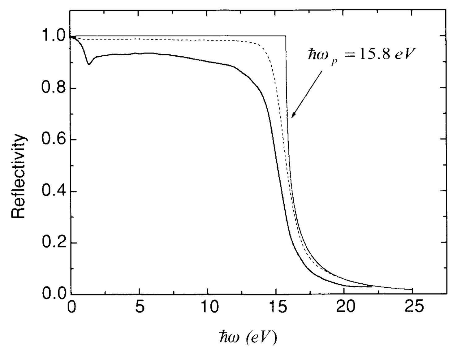
In this regime, the imaginary part of $ε$ is approximately zero and the real part has the well known form

\begin{array}{r} ε_{1} (ω) = 1 - \frac{ω_{p}^{2}}{ω^{2}}, \end{array}

such that the reflectivity drops drastically, from close to unity towards zero (compare with conceptual diagrams of reflectivity). Metals become nearly transparent in the range $ω > ω_{p}$ . In conceptual diagrams, one also notices the rapid increase in the penetration depth $δ$ , showing the transparency of the metal.

In all these considerations, we have neglected the contributions to the dielectric function due to the ion cores (core electrons and nuclei). This may be incorporated in the following approximate way:

\begin{array}{r} ε_{1} (ω) = ε_{\infty} - \frac{ω_{p}^{2}}{ω^{2}} . \end{array}

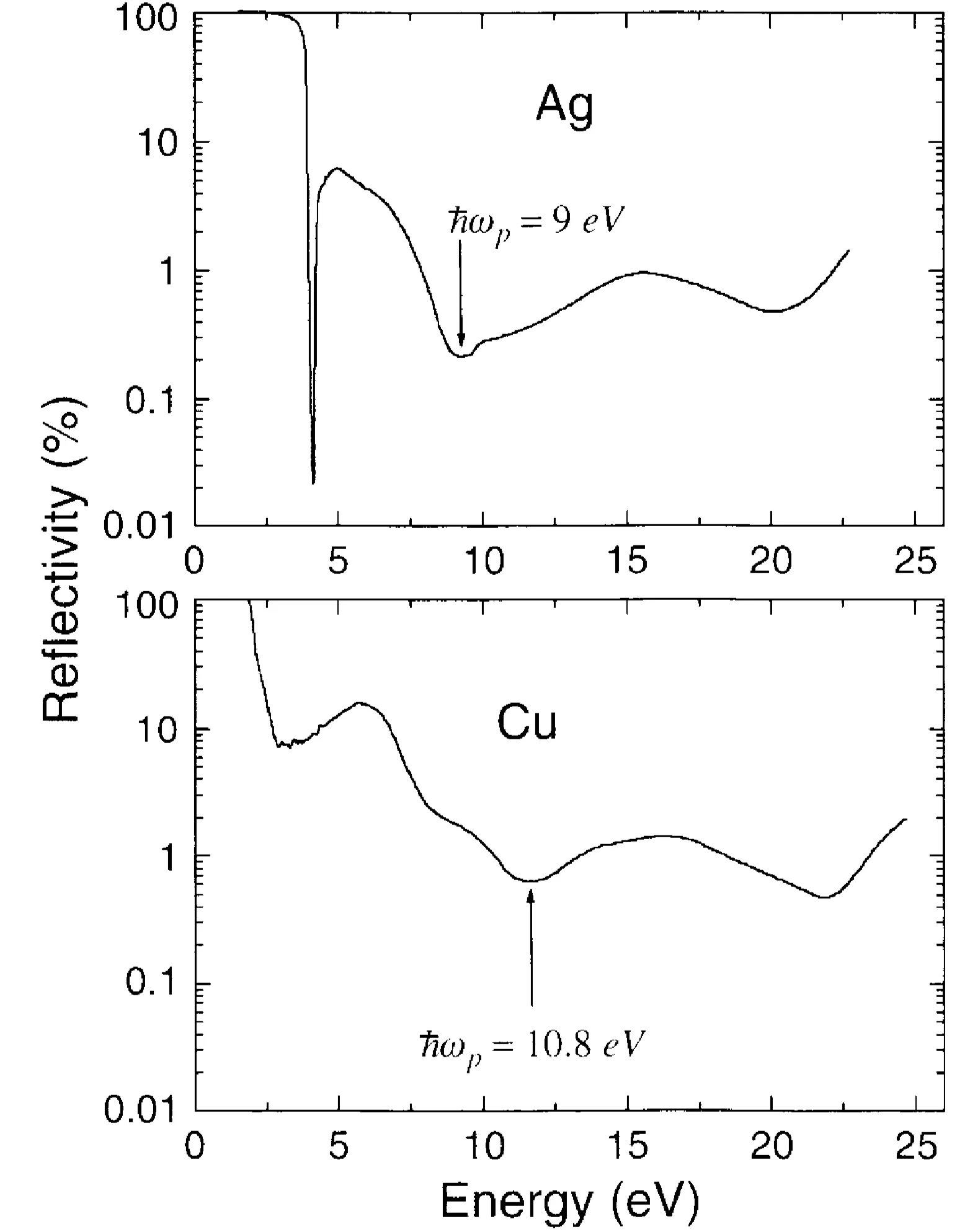
This influences the reflecting properties of metals; particularly, the value of $ω_{p}$ is reduced to $ω_{p}^{'} = ω_{p} / \sqrt{ε_{\infty}}$ , where $ε_{\infty}$ is the frequency-independent part of the dielectric function. With this, the reflectivity for frequencies above $ω_{p}^{'}$ approaches $R_{\infty} = {(\sqrt{ε_{\infty}} - 1)}^{2} / {(\sqrt{ε_{\infty}} + 1)}^{2}$ , and $0 < R_{\infty} < 1$ .

Colour of metals

The practically full reflectance for frequencies below $ω_{p}$ is a typical feature of metals. Since for most metals, the plasma frequency lies well above the range of visible light ( $ℏ ω = 1.5 - 3.5 eV$ ), they appear shiny to our eye. While most polished metal surfaces appear shiny white, like silver, there are some metals with a colour, like gold which is yellow and copper which is reddish. White shininess results from reflectance on the whole visible frequency range, while for coloured metals there is a certain threshold above which the reflectance drops and frequencies towards blue are not or much weaker reflected. In most cases this drop is not connected with the plasma frequency, but with light absorption due to interband transitions. Note that the single band metal which was used for the Drude theory does not allow for optical absorption apart from the plasma excitation. Interband transition play a particularly important role for the noble metals, Cu, Ag, and Au. For these metals, the reflectance drop is caused by the transition from the completely occupied $d$ -band to the partially filled $s$ -band, $3 d \to 4 s$ in case of Cu. For copper, this drop appears below $2.5 eV$ so that predominantly red light is reflected. For gold, this threshold frequency is slightly higher, but still in the visible, while for silver, it lies beyond the visible range. For all these cases, the plasma frequency is not so easily recognisable in the reflectance. On the other hand, aluminium shows a reflectance rather close to the expected behaviour. Also here, there is a small reduction of the reflection due to interband absorption. However, this effect is weak and the strong drop occurs at the plasma frequency of $ℏ ω_{p} = 15.8 eV$ . Like silver also polished aluminium is white shiny.

6.2.3 The Relaxation Time

By replacing the collision integral by a relaxation time approximation, we implicitly introduced a connection between the scattering rate $W (k, k^{'})$ and the relaxation time $τ$ . This relation,

\begin{array}{r} \frac{f (k) - f_{0} (k)}{τ (ϵ_{k})} = \int \frac{d^{3} k^{'}}{(2 π)^{3}} W (k, k^{'}) {f (k) - f (k^{'})} \end{array}

will be studied for an isotropic system, with elastic scattering, and a small external field $E$ . The solution of the linearised Boltzmann equation is of the form

\begin{array}{r} f (k) = f_{0} (k) + A (| k |) k \cdot E, \end{array}

such that

\begin{array}{r} f (k) - f (k^{'}) = A (| k |) (k - k^{'}) \cdot E . \end{array}

Without loss of generality, we define $\hat{z} ∥ k$ , and introduce the parametrisation of the angles $θ$ (polar angle of $E$ ) and $θ^{'}, ϕ^{'}$ (polar and azimuth angle of $k^{'}$ ), leading to

\begin{aligned} k \cdot E & = | k | | E | \cos θ \\ k \cdot k^{'} & = | k | | k^{'} | \cos θ^{'} \\ k^{'} \cdot E & = | k^{'} | | E | (\cos θ \cos θ^{'} + \sin θ \sin θ^{'} \cos ϕ^{'}) . \end{aligned}

For elastic scattering, $| k | = | k^{'} |$ , we obtain

\begin{array}{r} f (k) - f (k^{'}) = A (| k |) | k | | E | [\cos θ (1 - \cos θ^{'}) - \sin θ \sin θ^{'} \cos ϕ^{'}] . \end{array}

Inserting this into the right-hand side of the definition of the collision integral, the $ϕ^{'}$ -dependent part of the integration vanishes for an isotropic system, and we are left with

\begin{aligned} \frac{f (k) - f_{0} (k)}{τ (ϵ_{k})} & = \int d Ω_{k^{'}} [f (k) - f (k^{'})] W (k, k^{'}) \\ = A (| k |) | k | | E | \cos θ \int d Ω_{k^{'}} (1 - \cos θ^{'}) W (k, k^{'}) \\ = [f (k) - f_{0} (k)] \int d Ω_{k^{'}} (1 - \cos θ^{'}) W (k, k^{'}) . \end{aligned}

The factor $[f (k) - f_{0} (k)]$ can be dropped on both sides of the equation, resulting in

\begin{array}{r} \frac{1}{τ (ϵ_{k})} = \int \frac{d^{3} k^{'}}{(2 π)^{3}} W (k, k^{'}) (1 - \cos θ^{'}) \end{array}

where one should remember that, for elastic scattering, the quasi-particle energy $ϵ_{k} = ϵ_{k^{'}}$ is conserved in the collision process. The scattering probability $W (k, k^{'})$ accounts for this restriction. In the next few sections we discuss different scattering processes, looking at collision probabilities, relaxation times and the resulting conductivity and resistivity contributions.

6.3 Impurity Scattering

6.3.1 Potential Scattering

Every deviation from the perfect periodicity of the ionic lattice is a source of quasi-particle scattering, leading to the loss of their original momentum. Without translational invariance, the conservation of momentum is lost, the energy, however, is still conserved. Possible static scatterers are among others vacancies, dislocations, and impurity atoms. The scattering rate $W (k, k^{'})$ for a potential $\hat{V}$ can be determined applying Fermi's golden rule,

\begin{array}{r} W (k, k^{'}) = \frac{2 π}{ℏ} n_{imp} {| ⟨ k^{'} | \hat{V} | k ⟩ |}^{2} δ (ϵ_{k} - ϵ_{k^{'}}) . \end{array}

This corresponds to the first Born approximation in scattering theory. Note, that this approximation is insufficient to describe resonant scattering. By $n_{imp}$ we denote the density of impurities, assuming only one species of them. For small densities $n_{imp}$ , it is reasonable to neglect interference effects between different impurities. According to the derived relation for relaxation time, the relaxation time $τ$ of a quasi-particle with momentum $ℏ k$ is given by

\begin{aligned} \frac{1}{τ (ϵ_{k})} & = \frac{2 π}{ℏ} n_{imp} \int \frac{d^{3} k^{'}}{(2 π)^{3}} {| ⟨ k^{'} | \hat{V} | k ⟩ |}^{2} (1 - \hat{k} \cdot {\hat{k}}^{'}) δ (ϵ_{k} - ϵ_{k^{'}}) \\ = n_{imp} v_{k} \int \frac{d σ}{d Ω_{k^{'}}} (k, k^{'}) (1 - \hat{k} \cdot {\hat{k}}^{'}) d Ω_{k^{'}} . \end{aligned}

with the differential scattering cross section $d σ / d Ω_{k^{'}}$ and $\hat{k} = k / | k |$ . Here, we used the connection between Fermi's golden rule and the Born approximation:
The scattering of particles with momentum $ℏ k$ into the solid angle $d Ω_{k^{'}}$ around $k^{'}$ yields

\begin{aligned} W (k, k^{'}) d Ω_{k^{'}} & = \frac{2 π}{ℏ Ω} \sum_{k^{'} \in d Ω_{k^{'}}} {| ⟨ k^{'} | \hat{V} | k ⟩ |}^{2} δ (ϵ_{k} - ϵ_{k^{'}}) \\ = \frac{2 π}{ℏ} \int_{k^{'} \in d Ω_{k^{'}}} \frac{d^{3} k^{'}}{(2 π)^{3}} {| ⟨ k^{'} | \hat{V} | k ⟩ |}^{2} δ (ϵ_{k} - ϵ_{k^{'}}) \\ = \frac{2 π}{ℏ} \frac{d Ω_{k^{'}}}{(2 π)^{3}} \frac{| k |^{2}}{(d ϵ / d k)} {| ⟨ k^{'} | \hat{V} | k ⟩ |}^{2} = \frac{d Ω_{k^{'}}}{(2 π)^{2} ℏ v_{k}} | k |^{2} {| ⟨ k^{'} | \hat{V} | k ⟩ |}^{2} . \end{aligned}

The scattering per incoming particle current $j_{in} d σ (k, k^{'}) = W (k, k^{'}) d Ω_{k^{'}}$ determines the differential cross section (where $j_{i n} = v_{k} / Ω$ for one particle in volume $Ω$ )

\begin{array}{r} v_{k} \frac{d σ}{d Ω_{k^{'}}} (k, k^{'}) = \frac{Ω}{(2 π)^{2} ℏ} | k |^{2} {| ⟨ k^{'} | \hat{V} | k ⟩ |}^{2} . \end{array}

Note the difference in the expressions for the relaxation time $τ$ and for the lifetime $\tilde{τ}$ ,

\begin{array}{r} \frac{1}{\tilde{τ}} = \int \frac{d^{3} k^{'}}{(2 π)^{3}} W (k, k^{'}) \end{array}

given by Fermi's golden rule. The factor $(1 - \cos θ^{'})$ in the expression for $1 / τ$ gives more weight to backscattering $(θ^{'} \approx π)$ compared to forward scattering $(θ^{'} \approx 0)$ , since the former has more influence in impeding transport. This explains why $τ$ is also termed transport lifetime.

Assuming defects in the form of point charges $Z e$ , whose screened potential is

\begin{array}{r} ⟨ k^{'} | \hat{V} | k ⟩ = \frac{4 π Z e^{2}}{{| k - k^{'} |}^{2} + k_{TF}^{2}} . \end{array}

In the limit of very strong screening, $k_{TF} ≫ k_{F}$ , the differential cross section becomes independent of the deviation $(k - k^{'})$ , the transport and the usual lifetime become equal, $τ = \tilde{τ},$ and

\begin{array}{r} \frac{1}{τ} \approx \frac{π}{ℏ} N (ϵ_{F}) n_{imp} {(\frac{4 π Z e^{2}}{k_{TF}^{2}})}^{2} . \end{array}

With this, we are now able to determine the conductivity for scattering on Coulomb defects, assuming $s$ -wave scattering only. Then, since $τ (ϵ)$ depends weakly on energy, the Drude formula yields

\begin{array}{r} σ = \frac{e^{2} n τ (ϵ_{F})}{m} \end{array}

or, for the specific resistivity $ρ = 1 / σ$ ,

\begin{array}{r} ρ = \frac{m}{e^{2} n τ (ϵ_{F})} . \end{array}

Both $σ$ and $ρ$ are independent of temperature. This contribution is called the residual resistivity of a metal, which approaches zero for a perfect material. The temperature dependence of the resistivity is induced in other scattering processes like electron-phonon scattering and electron-electron scattering, which will be considered below. The so-called residual resistance ratio $R R R = R (T = 300 K) / R (T = 0)$ is an often used quantity to benchmark the quality of a material. It is defined as the ratio between the resistance $R$ at room temperature and the resistance at zero temperature. The bigger the $R R R$ , the better the quality of the material. The typical value of $R R R$ for common copper is $40 - 50$ , while the $R R R$ for very clean aluminium reaches values up to 20000.

6.3.2 Kondo Effect

There are impurity atoms inducing so-called resonant scattering. If the resonance occurs close to the Fermi energy, the scattering rate is strongly energy dependent, inducing a more pronounced temperature dependence of the resistivity. An important example is the scattering off magnetic impurities with a spin degree of freedom, yielding a dramatic energy dependence of the scattering rate. This problem was first studied by Kondo in 1964 in order to explain the peculiar minima in resistivity in some materials. The coupling between the local spin impurities $S_{i}$ at $R_{i}$ and the quasi-particle spin $s$ has the exchange form

\begin{aligned} {\hat{V}}_{K} & = \sum_{i} {({\hat{V}}_{K})}_{i} = J \sum_{i} {\hat{S}}_{i} \cdot \hat{s} (r) δ (r - R_{i}) \\ = J \sum_{i} ({\hat{S}}_{i}^{z} {\hat{s}}^{z} (r) + \frac{1}{2} {\hat{S}}_{i}^{+} {\hat{s}}^{-} (r) + \frac{1}{2} {\hat{S}}_{i}^{-} {\hat{s}}^{+} (r)) δ (r - R_{i}) \\ = \frac{J ℏ}{2 Ω} \sum_{k, k^{'}, i} [{\hat{S}}_{i}^{z} ({\hat{c}}_{k ↑}^{†} {\hat{c}}_{k^{'} ↑} - {\hat{c}}_{k ↓}^{†} {\hat{c}}_{k^{'} ↓}) + {\hat{S}}_{i}^{+} {\hat{c}}_{k ↓}^{†} {\hat{c}}_{k^{'} ↑} + {\hat{S}}_{i}^{-} {\hat{c}}_{k ↑}^{†} {\hat{c}}_{k^{'} ↓}] e^{- i (k - k^{'}) \cdot R_{i}} . \end{aligned}

Here, it becomes important that spin flip processes, which change the spin state of the impurity and that of the scattered electron, are enabled. The results for the scattering rate are presented here without derivation,

\begin{array}{r} W (k, k^{'}) \approx J^{2} S (S + 1) [1 + 2 J N (ϵ_{F}) \ln (\frac{D}{| ϵ_{k} - ϵ_{F} |})] \end{array}

where $D$ is the bandwidth and we have assumed that $J N (ϵ_{F}) ≪ 1$ . The relaxation time is found to be

\begin{array}{r} \frac{1}{τ (ϵ_{k})} \approx \frac{J^{2} S (S + 1)}{ℏ} N (ϵ_{k}) [1 + 2 J N (ϵ_{F}) \ln (\frac{D}{| ϵ_{k} - ϵ_{F} |})] . \end{array}

Note that $W (k, k^{'})$ does not depend on angle, meaning that the process is described by $s$ -wave scattering. The energy dependence is singular at the Fermi energy, indicating that we are not dealing with simple resonant potential scattering, but with a much more subtle many-particle effect involving the electrons very near the Fermi surface. The fact that the local spins $S_{i}$ can flip, makes the scattering centre dynamical, because the scatterer is constantly changing. The scattering process of an electron is influenced by previous scattering events, leading to the singularity at $ϵ_{F}$ . This cannot be described within the first Born approximation, but requires at least the second approximation or the full solution. As mentioned before, the resonant behaviour induces a strong temperature dependence of the conductivity. Indeed,

\begin{aligned} σ (T) & = \frac{e^{2} k_{F}^{3}}{6 π^{2} m} \int d ϵ \frac{1}{4 k_{B} T \cosh^{2} ((ϵ - ϵ_{F}) / (2 k_{B} T))} τ (ϵ) \\ \approx \frac{e^{2} n}{8 m k_{B} T} \int d \tilde{ϵ} \frac{τ (\tilde{ϵ} + ϵ_{F})^{- 1}}{\cosh^{2} (\tilde{ϵ} / (2 k_{B} T))} \\ \approx \frac{e^{2} n τ (ϵ_{F})}{m} [1 - c (J N (ϵ_{F}))^{2} (\ln (D / k_{B} T))^{2} \dots] \end{aligned}

A more direct evaluation from $1 / τ (ϵ_{F})$ and integrating $\partial f_{0} / \partial ϵ$ would be more appropriate for a first approximation. The result for conductivity is typically:

\begin{array}{r} ρ (T) \approx ρ_{0} + A J^{2} S (S + 1) [1 - 2 J N (ϵ_{F}) \ln (\frac{D}{k_{B} T})] . \end{array}

Usual contributions to the resistance, like electron-phonon scattering discussed below, typically decrease with temperature. The Kondo contribution to the resistivity increases with decreasing temperature (for antiferromagnetic $J > 0$ ), inducing a minimum in the total resistance. At even lower temperatures, the resistivity saturates. In reality, the conductivity saturates at a finite value when the temperature is lowered below a characteristic Kondo temperature $T_{K}$ ,

\begin{array}{r} k_{B} T_{K} = D e^{- 1 / (| J | N (ϵ_{F}))}, \end{array}

a characteristic energy scale of this system. The real behaviour of the conductivity at temperatures $T ≪ T_{K}$ is not accessible by simple perturbation theory. This regime, known as the Kondo problem, represents one of the most interesting correlation phenomena of many-particle physics.

6.4 Electron-Phonon Scattering

Even in perfect metals, the conductivity becomes non-zero at finite temperature. The thermally induced distortions of the lattice, phonons, act as fluctuating scattering centres. In the language of electron-phonon interaction, electrons are scattered via absorption and emission of phonons, which induce local fluctuations in volume (as discussed in Chapter 3). The corresponding coupling term was given in previously derived expressions and simplifies with the definition of the displacement field operator to

\begin{array}{r} H_{int} = 2 i \sum_{k, q, s} {\tilde{V}}_{q} \sqrt{\frac{ℏ}{2 ρ_{0} ω_{q}}} | q | ({\hat{b}}_{q} - {\hat{b}}_{- q}^{†}) {\hat{c}}_{k + q, s}^{†} {\hat{c}}_{k s} . \end{array}

The interaction is formally similar to the coupling between electrons and photons. The dominant processes consist of single-phonon processes, that is, the absorption or emission of one phonon. Energy and momentum are conserved, such that, for the scattering of an electron from momentum $k$ to $k^{'}$ due to the emission of a phonon with momentum $q$ , we have

\begin{aligned} k & = k^{'} + q + G, \\ ϵ_{k} & = ℏ ω_{q} + ϵ_{k^{'}} . \end{aligned}

Here, $ω_{q} = c_{s} | q |$ is the phonon spectrum, while the reciprocal lattice vector $G$ allows for scattering in nearby Brillouin zones. By this, the phase space available for scattering is strongly reduced, especially near the Fermi energy. Note that $ℏ ω_{q} \leq ℏ ω_{D} ≪ ϵ_{F}$ . In order to calculate the scattering rates, the matrix elements of the available processes,

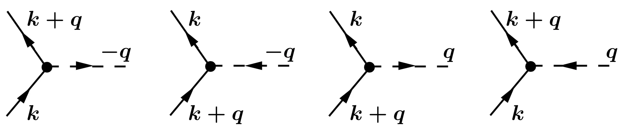
\begin{aligned} ⟨ k + q; N_{q^{'}} | ({\hat{b}}_{q} - {\hat{b}}_{- q}^{†}) {\hat{c}}_{k + q, s}^{†} {\hat{c}}_{k s} | k; N_{q^{'}}^{'} ⟩ = ⟨ k + q | {\hat{c}}_{k + q, s}^{†} {\hat{c}}_{k s} | k ⟩ & (\sqrt{N_{q^{'}}^{'}} δ_{N_{q^{'}}, N_{q^{'}}^{'} - 1} δ_{q, q^{'}} \\ - \sqrt{N_{q^{'}}^{'} + 1} δ_{N_{q^{'}}, N_{q^{'}}^{'} + 1} δ_{q, - q^{'}}) \end{aligned}

need to be calculated. In analogy to the discussion on electromagnetic radiation, the phenomenon of spontaneous phonon emission due to zero-point fluctuations appears. It is formally visible in the additional '+1' in the factors $(N_{\pm q} + 1)$ . From Fermi's golden rule we obtain

\begin{aligned} {(\frac{\partial f}{\partial t})}_{coll} = & - \frac{2 π}{ℏ} \sum_{q} | g (q) |^{2} [[f (k) (1 - f (k + q)) (N_{- q} + 1) \\ - f (k + q) (1 - f (k)) N_{- q}] δ (ϵ_{k + q} - ϵ_{k} + ℏ ω_{- q}) \\ - [f (k + q) (1 - f (k)) (N_{q} + 1) \\ - f (k) (1 - f (k + q)) N_{q}] δ (ϵ_{k + q} - ϵ_{k} - ℏ ω_{q})], \end{aligned}

where $g (q) = {\tilde{V}}_{q} | q | \sqrt{2 ℏ / (ρ_{0} ω_{q})}$ . Each of these four terms describes one of the single phonon scattering processes depicted here:

Attachments/Script 61.webp|700

The collision integral leads to a complicated integro-differential equation, whose solution is tedious and would involve the solution of the non-equilibrium phonon-problem as well. Instead of a full rigorous calculation including the non-equilibrium redistribution of phonons, we will consider the behaviour in various temperature regimes by an approximate treatment of the phonons. The characteristic temperature of phonons, the Debye temperature $Θ_{D} ≪ T_{F}$ , is much smaller than the Fermi temperature. Hence, the phonon energy is unimportant for the energy conservation, $ϵ_{k^{'} = k + q} \approx ϵ_{k}$ . Therefore we are allowed to impose momentum conservation $ϵ_{k + q} = ϵ_{k}$ and consider the lattice distortion as being essentially static, in the sense of an adiabatic Born-Oppenheimer approximation. The approximate collision integral then reads

\begin{array}{r} {(\frac{\partial f}{\partial t})}_{coll} = \frac{2 π}{ℏ} \sum_{q} | g (q) |^{2} 2 N (ω_{q}) [f (k + q) - f (k)] δ (ϵ_{k + q} - ϵ_{k}) \end{array}

where we assume the occupation of phonon states according to the equilibrium distribution for bosons,

\begin{array}{r} N (ω_{q}) = \frac{1}{e^{ℏ ω_{q} / k_{B} T} - 1} . \end{array}

This approximation includes all important aspects of the electron-phonon scattering we need to derive the temperature dependence of $ρ (T)$ .
In analogy to previous approaches, we obtain with relaxation-time Ansatz

\begin{array}{r} \frac{1}{τ (ϵ_{k})} = \frac{2 π}{ℏ} \frac{λ}{N (ϵ_{F})} \int \frac{d^{3} q}{(2 π)^{3}} ℏ ω_{q} N (ω_{q}) (1 - \cos θ) δ (ϵ_{k + q} - ϵ_{k}) \end{array}

where $| k | = | k + q | = k_{F}$ , meaning that only the electrons in a thin shell close to the Fermi surface are relevant. Furthermore, we parameterised $g (q)$ according to

\begin{array}{r} | g (q) |^{2} = \frac{λ}{2 N (ϵ_{F}) Ω} ℏ ω_{q}, \end{array}

where $λ$ is a dimensionless electron-phonon coupling constant. In usual metals $λ < 1$ . As in the case of defect scattering, the relaxation time depends only weakly on the electron energy. But, unlike previously, the direct temperature dependence enters via the dependence on temperature of the phonon occupation $N (ω_{q})$ .

Attachments/Script 62.webp|700

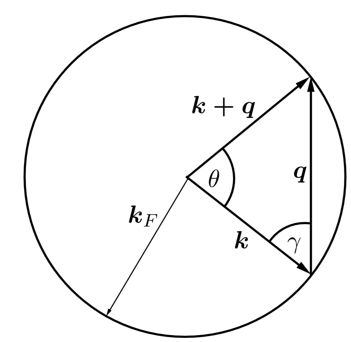
In order to perform the integration in the expression for $1 / τ$ , we have to re-express $δ (ϵ_{k + q} - ϵ_{k})$ by writing (with $q = | q |, k_{F} = | k_{F} |$ ):

\begin{aligned} δ (ϵ_{k + q} - ϵ_{k}) & = δ (\frac{ℏ^{2}}{2 m} (q^{2} - 2 k_{F} q \cos γ)) \\ = \frac{m}{ℏ^{2} k_{F} q} δ (\frac{q}{2 k_{F}} - \cos γ) \end{aligned}

where $γ$ is defined in the relevant geometry. From there, we also see that $2 γ + θ = π$ , and thus, find the relation

\begin{array}{r} 1 - \cos θ = 1 + \cos (2 γ) = 2 \cos^{2} (γ) . \end{array}

Obviously, we have to integrate $q$ over the range $[0, 2 k_{F}]$ on the right-hand side of the expression for $1 / τ$ , which can be reformulated to

\begin{aligned} \frac{1}{τ (ϵ_{F}, T)} & = \frac{- λ}{N (ϵ_{F})} \frac{m}{ℏ^{2} π k_{F}} \int_{0}^{2 k_{F}} d q q ω_{q} N (ω_{q}) \int_{0}^{π / 2} d γ \sin γ \cos^{2} (γ) δ (\frac{q}{2 k_{F}} - \cos γ) \\ = \frac{λ}{4 N (ϵ_{F})} \frac{m c_{s}}{ℏ^{2} π k_{F}^{3}} \int_{0}^{2 k_{F}} \frac{q^{4} d q}{e^{ℏ c_{s} q / k_{B} T} - 1} \\ = \frac{λ}{4 N (ϵ_{F})} \frac{m c_{s} k_{F}^{2}}{ℏ^{2} π} {(\frac{T}{Θ_{D}})}^{5} \int_{0}^{2 Θ_{D} / T} \frac{y^{4} d y}{e^{y} - 1}, \end{aligned}

where we have approximated the Debye temperature by $k_{B} Θ_{D} \approx ℏ c_{s} k_{F}$ . We notice the two distinct characteristic temperature regimes,

\begin{array}{r} \frac{1}{τ} = {\begin{cases} 6 ζ (5) λ π \frac{k_{B} Θ_{D}}{ℏ} {(\frac{T}{Θ_{D}})}^{5}, & T ≪ Θ_{D} \\ λ π \frac{k_{B} Θ_{D}}{ℏ} (\frac{T}{Θ_{D}}), & T ≫ Θ_{D} \end{cases} . \end{array}

The prefactors depend on the details of the approximation, whereas the qualitative temperature dependence does not. We finally obtain the conductivity and resistivity from the formula for conductivity,

\begin{aligned} σ & = \frac{e^{2} n}{m} τ (T) \\ ρ & = \frac{m}{e^{2} n} \frac{1}{τ (T)} \end{aligned}

where we used the weak energy dependence of $τ (ϵ \approx ϵ_{F}, T)$ . With this, we obtain the well-known Bloch-Grüneisen form

\begin{array}{r} ρ (T) \sim {\begin{cases} T^{5}, & T ≪ Θ_{D} \\ T, & T ≫ Θ_{D} . \end{cases} \end{array}

At high temperatures, $ρ$ is determined by the occupation of phonon states

\begin{array}{r} N (ω_{q}) \approx \frac{k_{B} T}{ℏ ω_{q}} \end{array}

which change the scattering strength (amplitude) of the lattice modulation linear in $T$ . At low temperature only the lowest phonon states are occupied $ℏ ω_{q} < k_{B} T$ yield $| q | < k_{B} T / (ℏ c_{s})$ . Thus, at low temperatures only long-wave length modulations of the lattice generate a scattering potentials which deflects electrons only slightly from their trajectories (forward scattering dominates). This represents a restriction of the scattering phase space becoming ever smaller with decreasing temperature.

6.5 Electron-Electron Scattering

In Chapter 5 we learned that, taking a short-ranged electron-electron interaction into account, scattering rate for electrons decreases strongly close to the Fermi surface. The basic reason for this lies in the constraint of the scattering phase space imposed by the Pauli principle. The lifetime, which we identify with the relaxation time here, has the form

\begin{array}{r} \frac{1}{τ (ϵ)} = \frac{1}{τ_{e}} {(\frac{ϵ}{ϵ_{F}} - 1)}^{2} \end{array}

where energy and momentum conservation is taken into account and $τ_{e}$ is a constant of unit time. We may now calculate the mean relaxation time $\bar{τ}$ as introduced in Section 6.2.2. To regularise the integrals we take here also impurity scattering into account by adding a constant to the scattering rate and obtain for the resistivity

\begin{array}{r} ρ (T) = ρ_{0} + \frac{π^{2}}{3} \frac{m}{n e^{2} τ_{e}} {(\frac{k_{B} T}{ϵ_{F}})}^{2} . \end{array}

Calculation of mean scattering time $\bar{τ}$ : We use Matthiessen's rule to add the scattering rates of electron-electron and impurity scattering to the form

\begin{array}{r} \frac{1}{τ (ϵ)} = \frac{1}{τ_{e}} {(\frac{ϵ}{ϵ_{F}} - 1)}^{2} + \frac{1}{τ_{0}} . \end{array}

Restricting to the small temperature limit, we determine $\bar{τ}$ by

\begin{aligned} \bar{τ} & = - \int d ϵ τ (ϵ) \frac{\partial f_{0}}{\partial ϵ} = \int_{- \infty}^{+ \infty} d E \frac{τ (E)}{4 k_{B} T \cosh^{2} (E / (2 k_{B} T))} \\ \approx \int_{- \infty}^{+ \infty} d E \frac{1}{4 k_{B} T \cosh^{2} (E / (2 k_{B} T))} {τ_{0} - \frac{τ_{0}^{2}}{τ_{e}} \frac{E^{2}}{ϵ_{F}^{2}}} \\ = τ_{0} - \frac{π^{2}}{3} \frac{τ_{0}^{2}}{τ_{e}} {(\frac{k_{B} T}{ϵ_{F}})}^{2} \end{aligned}

where $E = ϵ - ϵ_{F}$ . The resistivity is given by

\begin{array}{r} ρ (T) = \frac{m}{n e^{2} \bar{τ} (T)} \approx \frac{m}{n e^{2} τ_{0}} {1 + \frac{π^{2}}{3} \frac{τ_{0}}{τ_{e}} {(\frac{k_{B} T}{ϵ_{F}})}^{2}} \end{array}

and with $ρ_{0} = m / (n e^{2} τ_{0})$ as the residual resistivity leads to $ρ (T)$ .
Electron-electron scattering introduces a quadratic temperature dependence to resistivity. This is a key property of a Fermi liquid and is often considered an identifying criterion.

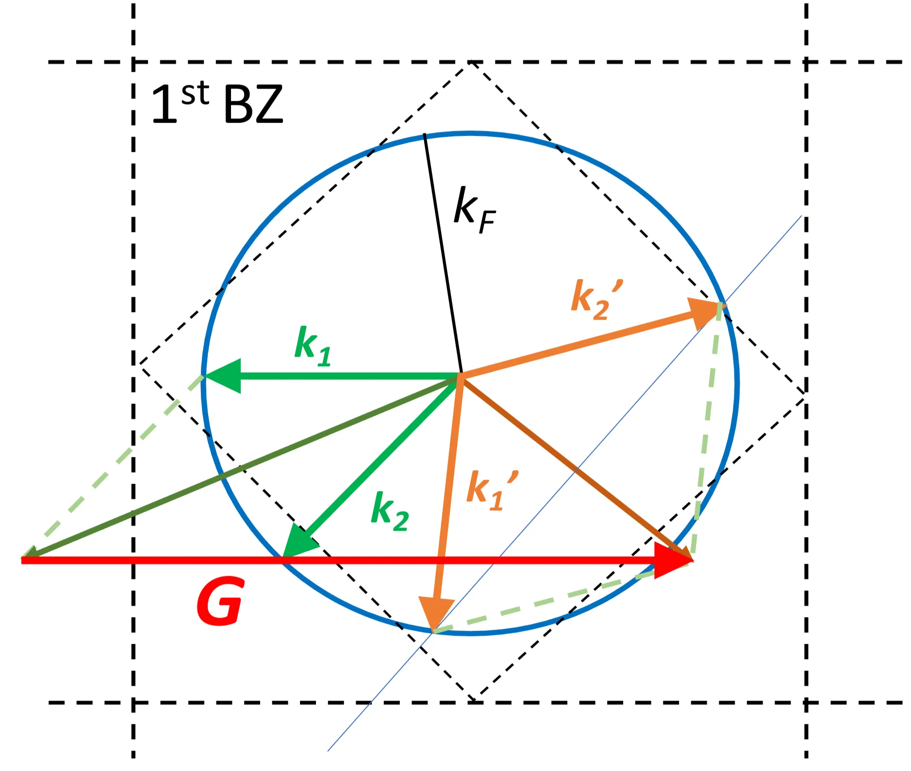
Umklapp process

We should here also address the problem of momentum relaxation through electron-electron scattering. Actually in every electron-electron scattering process the total momentum is conserved,

\begin{array}{r} k_{1} + k_{2} = k_{1}^{'} + k_{2}^{'} . \end{array}

The situation is even more constraint through the fact that all momenta lie essentially on the Fermi surfaces, $| k_{i} | \approx k_{F}$ . In this way electron-electron scattering could not contribute to momentum relaxation and would not enter the discussion of resistivity, unlike we have done above.
The short-coming of our argument is that the momentum conservation as given in this form is only valid in a completely translational system. It is necessary consider the effect of the ion lattice, such that we actually deal here with lattice momenta $k$ . Under this condition the "momentum conservation" involves also reciprocal lattice vectors,

\begin{array}{r} k_{1} + k_{2} + G = k_{1}^{'} + k_{2}^{'} \end{array}

which connects different Brillouin zones, as shown here:

Attachments/Script 63.webp|700

In this way momentum can be transferred to the lattice. Still the conditions are constraint by the fact that all electron momenta lie on the Fermi surface. Such processes are termed Umklapp scattering and play an important role in electron-phonon scattering as well.

6.6 Matthiessen's Rule and the Ioffe-Regel Limit

Matthiessen's rule states, that the scattering rates of different scattering processes can simply be added, leading to

\begin{array}{r} W (k, k^{'}) = W_{1} (k, k^{'}) + W_{2} (k, k^{'}) \end{array}

or, expressed in the relaxation time approximation,

\begin{array}{r} \frac{1}{τ} = \frac{1}{τ_{1}} + \frac{1}{τ_{2}} \end{array}

and

\begin{array}{r} ρ = \frac{m}{n e^{2} τ} = \frac{m}{n e^{2}} (\frac{1}{τ_{1}} + \frac{1}{τ_{2}}) = ρ_{1} + ρ_{2} . \end{array}

This rule is not a theorem and corresponds effectively to a serial coupling of resistors in a classical circuit. It is applicable, if the different scattering processes are independent. Actually, the assumption that the impurity scattering rate depends linearly on the impurity density $n_{imp}$ is already an application of Matthiessen's rule. Mutual influences of impurities, for example, through interference effects due to the coherent scattering of an electron at different impurities, would invalidate this simplification. An example where Matthiessen's rule is violated is a one-dimensional system, where a single scatterer $i$ induces a finite resistance $R_{i}$ . Two serial scatterers then lead to a total resistance

\begin{array}{r} R = R_{1} + R_{2} + \frac{2 e^{2}}{h} R_{1} R_{2} \geq R_{1} + R_{2} . \end{array}

The reason is, that in one-dimensional systems, the interference of backscattered waves is unavoidable and no impurity can be treated as isolated. Furthermore, every particle traversing the whole system has to pass all scatterers. The more general Matthiessen's rule,

\begin{array}{r} ρ \geq ρ_{1} + ρ_{2} \end{array}

is still valid. Another source of deviation from Matthiessen's rule arises, if the relaxation time depends on $k$ , since then the averaging is not the same for all scattering processes. The electron-phonon coupling can be modified by the scattering on impurities, most importantly in the presence of anisotropic Fermi surfaces. For the analysis of resistance data of simple metals, we often assume the validity of Matthiessen's rule. A typical example is the resistance minimum explained by Kondo, where

\begin{aligned} ρ (T) & = ρ_{0} + ρ_{e - p} (T) + ρ_{K} (T) + ρ_{e - e} (T) \\ = ρ_{0} + α T^{5} + β (1 + 2 J N (ϵ_{F}) \ln (D / k_{B} T)) + γ T^{2}, \end{aligned}

where $α, β$ , and $γ$ are numerical constants. Upon decreasing temperature, the Kondo term is increasing, whereas the electron-phonon and electron-electron contributions decrease. Consequently, there is a minimum.

We now turn to the discussion of resistivity in the high-temperature limit. Believing the previous considerations entirely, the electrical resistivity would grow indefinitely with temperature. In most cases, however, the resistivity will saturate at a finite limiting value. We can understand this from simple considerations writing the mean free path $ℓ = v_{F} τ (ϵ_{F})$ as the mean distance an electron travels freely between two collisions. The lattice constant $a$ is a natural lower boundary to $ℓ$ in the crystal lattice. Furthermore, we assumed so far that scattering occurs between two states with sharp momenta $k$ and $k^{'}$ . If the de Broglie wavelength becomes comparable to the mean free path, the framework becomes unfounded and $k_{F}^{- 1}$ would become a boundary for $ℓ$ . In most systems $a$ and $k_{F}^{- 1}$ are comparable lengths. Empirically, the resistivity is described via the formula

\begin{array}{r} \frac{1}{ρ (T)} = \frac{1}{ρ_{B T} (T)} + \frac{1}{ρ_{max}} \end{array}

corresponding to the parallel addition of two resistivities; on one hand, $ρ_{B T} (T)$ , which we have investigated using the Boltzmann transport theory, and on the other hand the limiting value $ρ_{max}$ . This is in clear disagreement to Matthiessen's rule, which is to be expected, since for $k_{F} ℓ \sim 1$ , complex interference effects will arise. The saturated resistivity $ρ_{max}$ can be estimated from the Jellium model,

\begin{aligned} ρ_{max} & = \frac{m}{e^{2} n τ (ϵ_{F})} = \frac{3 π^{2} m}{e^{2} k_{F}^{3} τ (ϵ_{F})} = \frac{h}{e^{2}} \frac{3 π}{2 k_{F}^{2} ℓ} \\ \sim \frac{h}{e^{2}} \frac{3 π}{2 k_{F}} \end{aligned}

where we used $ℓ^{- 1} \sim k_{F}$ . For a typical value $k_{F} \sim 10^{8} {cm}^{- 1}$ of the Fermi wave vector, we find $ρ_{max} \sim 1 m Ω cm$ , which is called the Ioffe-Regel limit. Establishing a quantitative estimate of $ρ_{max}$ for a given material is often difficult. There are even materials whose resistivity surpasses the Ioffe-Regel limit.

6.7 General Transport Coefficients

Simultaneously with charge, electrons will also transport energy, that is, heat and entropy. This is why charge and heat transport are naturally interconnected. In the following, we generalise the transport theory set up above to include this interplay.

6.7.1 Generalised Boltzmann Equation

We consider a metal with weakly space-dependent temperature $T (r)$ and chemical potential $μ (r)$ . The distribution function then reads

\begin{array}{r} δ f (k; r) = f (k; r) - f_{0} (k, T (r), μ (r)), \end{array}

where

\begin{array}{r} f_{0} (k, T (r), μ (r)) = \frac{1}{e^{(ϵ_{k} - μ (r)) / k_{B} T (r)} + 1} . \end{array}

In addition, we require the charge density to remain constant in space, that is,

\begin{array}{r} \int \frac{d^{3} k}{(2 π)^{3}} f (k; r) = n_{0} \end{array}

for all $r$ . In this section, we introduce the electro-chemical potential for electrons $η (r) = - e ϕ (r) + μ (r)$ generating the general force field $E = - \nabla η = - \nabla (- e ϕ + μ)$ , where $ϕ (r)$ denotes the electrostatic potential which produces the electric field $E = - \nabla ϕ$ such that $E = - e E - \nabla μ$ . With this, the Boltzmann equation for the stationary situation reads

\begin{aligned} {(\frac{\partial f}{\partial t})}_{coll} & = v_{k} \cdot \nabla_{r} f + \dot{k} \cdot \nabla_{k} f \\ = - \frac{\partial f}{\partial ϵ_{k}} v_{k} \cdot (\frac{ϵ_{k} - μ}{T} \nabla_{r} T - E) . \end{aligned}

Attachments/Script 64.webp|700

In the relaxation time approximation for the collision integral, we obtain the solution

\begin{array}{r} δ f (k) = - \frac{\partial f_{0}}{\partial ϵ_{k}} τ (ϵ_{k}) v_{k} \cdot (E - \frac{ϵ_{k} - μ}{T} \nabla_{r} T), \end{array}

which allows us to calculate the charge and heat currents,

\begin{aligned} J_{e} & = - 2 e \int \frac{d^{3} k}{(2 π)^{3}} v_{k} δ f (k) \\ J_{q} & = 2 \int \frac{d^{3} k}{(2 π)^{3}} (ϵ_{k} - μ) v_{k} δ f (k) \end{aligned}

respectively. One could be tempted to use

\begin{array}{r} J_{q} = 2 \int \frac{d^{3} k}{(2 π)^{3}} ϵ_{k} v_{k} δ f (k) \end{array}

for the heat current. However, $ϵ_{k}$ relates to the internal energy. Considering the specific heat, we obtain for the heat

\begin{array}{r} δ Q = C (T) d T = \frac{2}{Ω} \sum_{k} \frac{\partial f_{0} (ϵ_{k})}{\partial T} (ϵ_{k} - μ) d T \end{array}

which shows that heat involves $ϵ_{k} - μ$ including the chemical potential. Inserting the solution for $δ f (k)$ into the two definitions above yields

\begin{aligned} J_{e} & = - e {\hat{K}}^{(0)} E - \frac{e}{T} {\hat{K}}^{(1)} (- \nabla T) \\ J_{q} & = + {\hat{K}}^{(1)} E + \frac{1}{T} {\hat{K}}^{(2)} (- \nabla T) \end{aligned}

where $\nabla$ should be understood as $\nabla_{r}$ and the tensors ${\hat{K}}^{(n)} (n \in N_{0})$ are defined as

\begin{array}{r} K_{α β}^{(n)} = - \frac{1}{4 π^{3}} \int d ϵ \frac{\partial f_{0}}{\partial ϵ} τ (ϵ) (ϵ - μ)^{n} \int d Ω_{k} \frac{v_{F α k} v_{F β k}}{ℏ | v_{F} |} | k_{F} |^{2} . \end{array}

For an isotropic system these transport coefficients are no longer tensors but represented by scalars,

\begin{array}{r} K^{(n)} = - \frac{n_{0}}{m} \int d ϵ \frac{\partial f_{0}}{\partial ϵ} τ (ϵ) (ϵ - μ)^{n} . \end{array}

In the case $T ≪ T_{F}$ we can calculate the coefficients,

\begin{aligned} K^{(0)} (ϵ_{F}) & = \frac{n_{0} (ϵ_{F}) τ (ϵ_{F})}{m} \\ K^{(1)} (ϵ_{F}) & = {\frac{π^{2}}{3} {(k_{B} T)}^{2} \frac{\partial}{\partial ϵ} K^{(0)} (ϵ) |}_{ϵ = ϵ_{F}} \\ K^{(2)} (ϵ_{F}) & = \frac{π^{2}}{3} {(k_{B} T)}^{2} K^{(0)} (ϵ_{F}) . \end{aligned}

Note, we used that if a function $g (ϵ)$ depends only weakly on $ϵ$ in the vicinity of $ϵ_{F}$ , we can use the Sommerfeld expansion to derive a general approximation for following integrals

\begin{array}{r} - \int d ϵ g (ϵ) \frac{\partial f_{0}}{\partial ϵ} = g (ϵ_{F}) + {\frac{π^{2}}{6} {(k_{B} T)}^{2} \frac{\partial^{2} g (ϵ)}{\partial ϵ^{2}} |}_{ϵ = ϵ_{F}} + \dots \end{array}

and

\begin{array}{r} - \int d ϵ g (ϵ) (ϵ - ϵ_{F}) \frac{\partial f_{0}}{\partial ϵ} = {\frac{π^{2}}{3} {(k_{B} T)}^{2} \frac{\partial g (ϵ)}{\partial ϵ} |}_{ϵ = ϵ_{F}} + \dots, \end{array}

in the limit $T \to 0$ . We used that $μ \to ϵ_{F}$ in that asymptotic case.

We measure the electrical resistivity assuming $\nabla T = \nabla μ = 0$ for all $r$ . With this, we find the expression

\begin{array}{r} σ (ϵ_{F}) = e^{2} K^{(0)} (ϵ_{F}) = \frac{e^{2} n_{0} (ϵ_{F}) τ (ϵ_{F})}{m} . \end{array}

In order to determine the thermal conductivity $\hat{κ}$ relating the heat current $J_{q}$ to $\nabla T$ when no external electric field $E$ is applied, we set $J_{e} = 0$ as for an open circuit. Then, the expressions for charge and heat current reveal the appearance of an general force field

\begin{array}{r} E = \frac{K^{(1)}}{T K^{(0)}} \nabla T . \end{array}

Thus, the heat current is given by

\begin{array}{r} J_{q} = - \frac{1}{T} (K^{(2)} - \frac{(K^{(1)})^{2}}{K^{(0)}}) \nabla T = - κ \nabla T . \end{array}

In simple metals, the second term in the expression for thermal conductivity is often negligible as compared to the first one and we obtain in this case

\begin{array}{r} κ = \frac{1}{T} K^{(2)} = \frac{π^{2} k_{B}^{2}}{3} T K^{(0)} = \frac{π^{2}}{3} \frac{k_{B}^{2}}{e^{2}} T σ, \end{array}

which is the well-known Wiedemann-Franz law. Note, that we can write the thermal conductivity in the form

\begin{array}{r} κ = \frac{C}{e^{2} N (ϵ_{F})} σ \end{array}

where $C = π^{2} N (ϵ_{F}) k_{B}^{2} T / 3$ denotes the electronic specific heat (per unit volume if $N (ϵ_{F})$ is per unit volume).

6.7.2 Thermoelectric Effect

The relation for the induced electrochemical field gradient shows, that a temperature gradient induces an electric field. For a simple, isotropic system, this relation reduces to

\begin{array}{r} E = - e Q \nabla T = \frac{K^{(1)}}{T K^{(0)}} \nabla T \end{array}

with the Seebeck coefficient

\begin{array}{r} Q = - {\frac{π^{2}}{3} \frac{k_{B}^{2} T}{e} \frac{σ^{'} (ϵ)}{σ (ϵ)} |}_{ϵ = ϵ_{F}} . \end{array}

This is the so-called Mott formula which looses its validity at high-temperatures or very anisotropic scattering. Using $σ (ϵ) = n (ϵ) e^{2} τ (ϵ) / m$ , we investigate $σ^{'} (ϵ)$ ,

\begin{array}{r} σ^{'} (ϵ) = \frac{τ^{'} (ϵ)}{τ (ϵ)} σ (ϵ) + \frac{n^{'} (ϵ)}{n (ϵ)} σ (ϵ) = \frac{τ^{'} (ϵ)}{τ (ϵ)} σ (ϵ) + \frac{N (ϵ)}{n (ϵ)} σ (ϵ) \end{array}

and obtain an additional contribution to $Q$ , if the relaxation time depends strongly on energy. This is most prominent in collision processes in which resonant scattering is involved (for example, the Kondo effect). In the opposite situation, namely, when the first term is irrelevant, the Seebeck coefficient

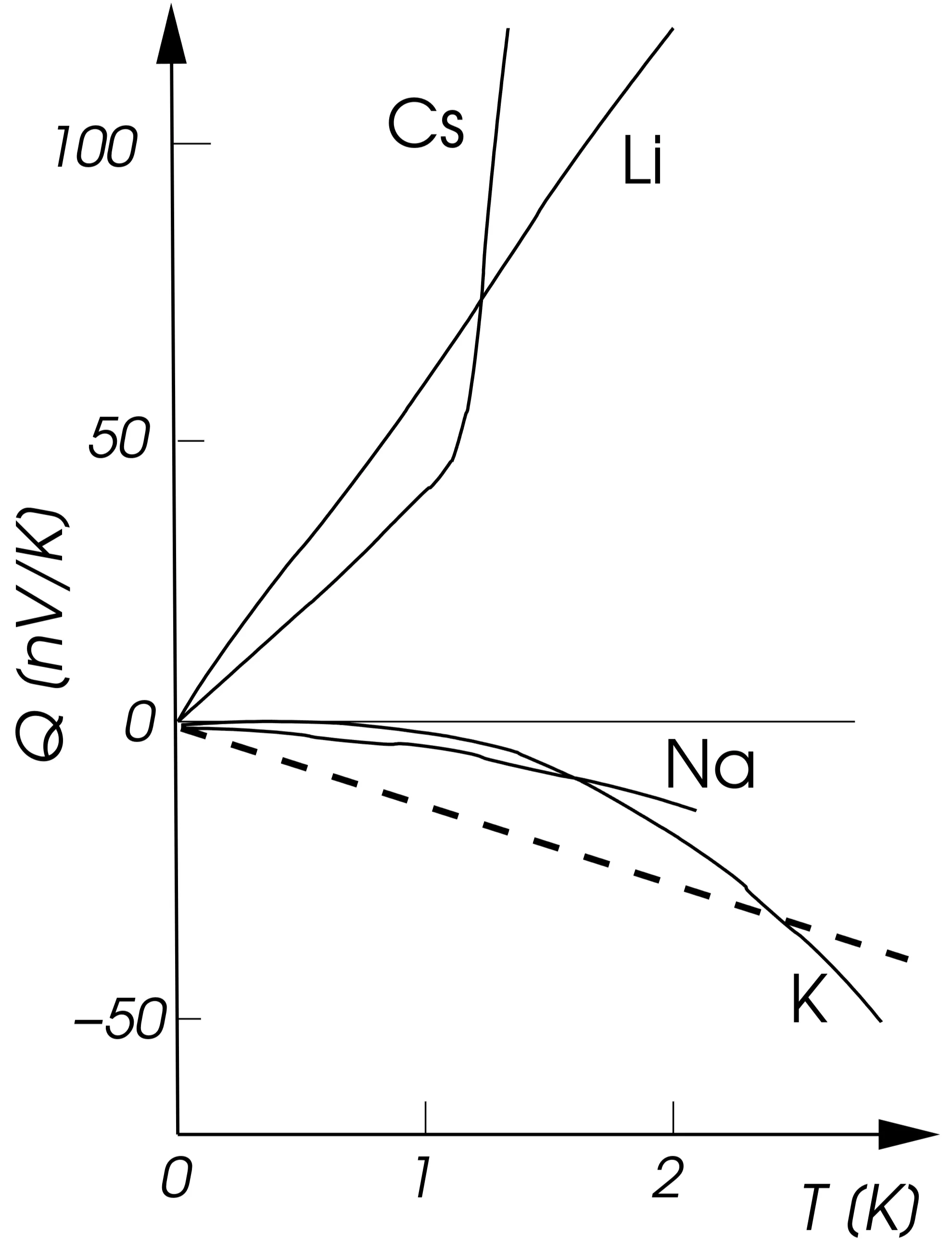
\begin{array}{r} Q = - \frac{π^{2}}{3} \frac{k_{B}^{2} T}{e} \frac{N (ϵ_{F})}{n (ϵ_{F})} = - \frac{S}{n e} \end{array}

is simply reduced to the entropy per electron (per unit charge). For simple metals such as the alkali metals we may estimate the low-temperature values using this expression

\begin{array}{r} Q = - \frac{π^{2}}{2} \frac{k_{B}^{2} T}{e ϵ_{F}} = - \frac{π^{2}}{2} \frac{k_{B} T}{e T_{F}} \end{array}

which for $T_{F} (Na, K) \approx 3 \times 10^{4} K$ leads to $Q \approx - 1.4 \times (T / K) nV K^{- 1}$ .
A comparison with experiments shows that the order of magnitude works reasonably well for Na and K. However, for Li and Cs even the sign is different. Differences occur through phonon effects, such as the so-called phonon drag which we have neglected here:

Attachments/Script 65.webp|700

In the following, we consider two different types of thermoelectric effects.

Seebeck effect

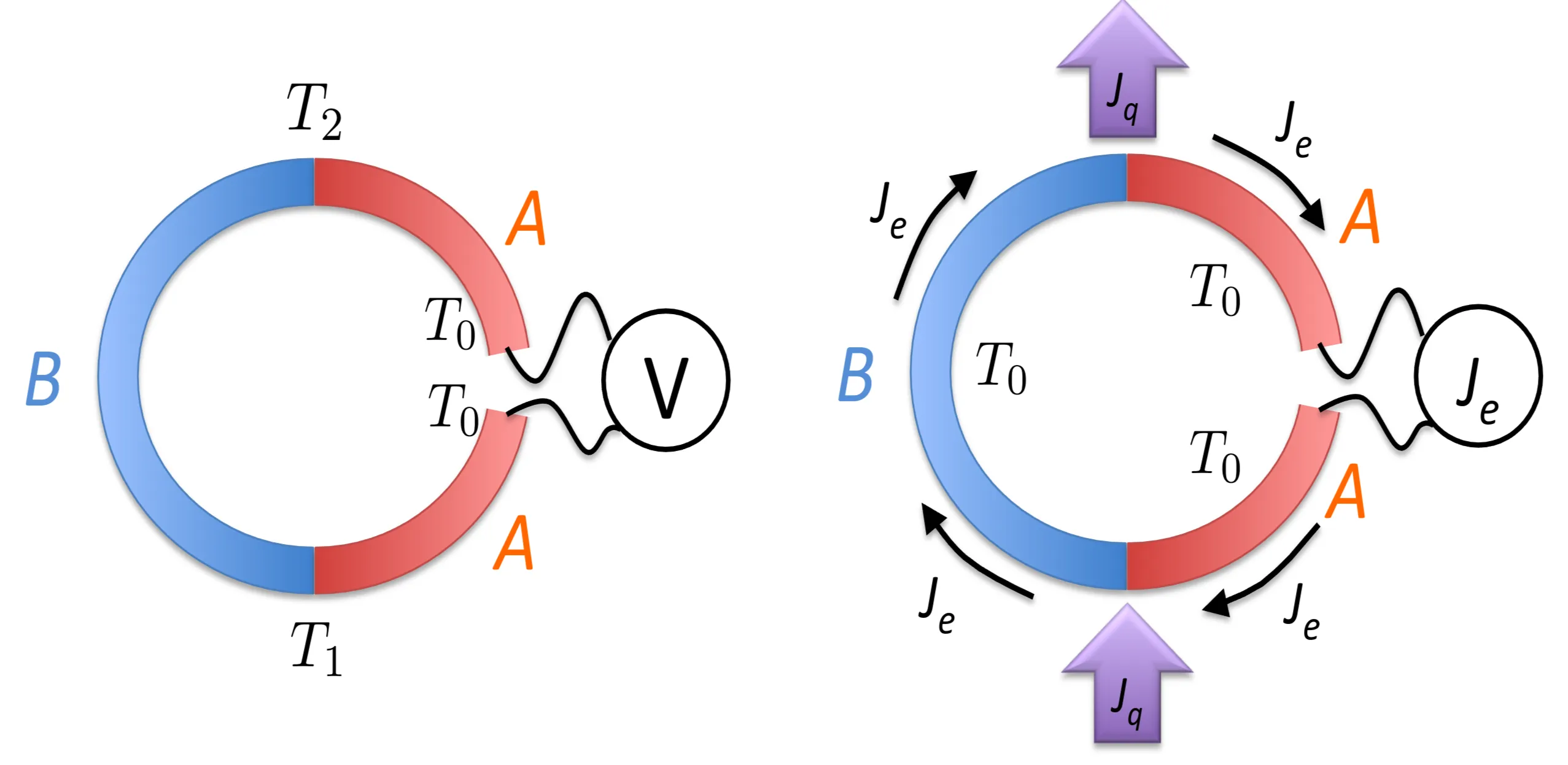
The first is the Seebeck effect, where a thermoelectric voltage appears in a bi-metallic system (compare with the conceptual diagram). With the relation $E = - e Q \nabla T$ , a temperature gradient across metal $B$ induces a voltage

\begin{aligned} V & = - \frac{1}{e} \int d l \cdot E \\ = Q_{A} \int_{T_{0}}^{T_{1}} d l \cdot \nabla T + Q_{B} \int_{T_{1}}^{T_{2}} d l \cdot \nabla T + Q_{A} \int_{T_{2}}^{T_{0}} d l \cdot \nabla T \\ = (Q_{B} - Q_{A}) (T_{2} - T_{1}) . \end{aligned}

The resulting voltage $V$ appears between the two ends of a second metal $A$ , whose contacts are kept at the same temperature $T_{0}$ . The integral of $\nabla μ$ along the whole path vanishes since the temperature at both ends of metal $A$ is the same $T_{0}$ . Here, a bi-metallic configuration was chosen to reveal voltage differences across the contacts which are absent in a single metal.

Peltier effect

The second phenomenon, termed Peltier effect, emerges in a system kept at the same temperature everywhere. Here, an electric current $J_{e}$ between the two contacts of the metal $A$ induces a heat current in the bi-metallic system, such that heat is transferred from one reservoir (top) to another (bottom):

Attachments/Script 66.webp|700

This follows from the general transport equations by assuming $\nabla T = 0$ , where

\begin{aligned} J_{e} & = e^{2} K^{(0)} E \\ J_{q} & = - e K^{(1)} E \end{aligned}

implies (for isotropic systems)

\begin{array}{r} J_{q} = - \frac{K^{(1)}}{e K^{(0)}} J_{e} = Π J_{e} = Q T J_{e} . \end{array}

The coupling $Π = T Q$ between $J_{q}$ and $J_{e}$ is called Peltier coefficient. According to the diagram, a contribution to the heat current is to be expected from both metals $A$ and $B$ ,

\begin{array}{r} J_{q} = (Π_{A} - Π_{B}) J_{e} = T_{0} (Q_{A} - Q_{B}) J_{e} . \end{array}

This means, that the heat transfer between reservoirs can be controlled by electrical current. It has to be emphasized here that the bi-metal design of the devices described serves the observation of the two effects which both represent bulk effects of the two metals A and B. By no means should it be mistaken as an effect originating from the inter-metal contacts.

6.8 Anderson Localisation in One-Dimensional Systems

Transport in one spatial dimension is very special, since there are only two different directions to go: forward and backward. We introduce the transfer matrix formalism and use it to express the conductivity through the Landauer formula. We will then investigate the effects of multiple scattering at different obstacles, leading to the so-called Anderson localisation, which turns a metal into an insulator.

6.8.1 Landauer Formula for a Single Impurity

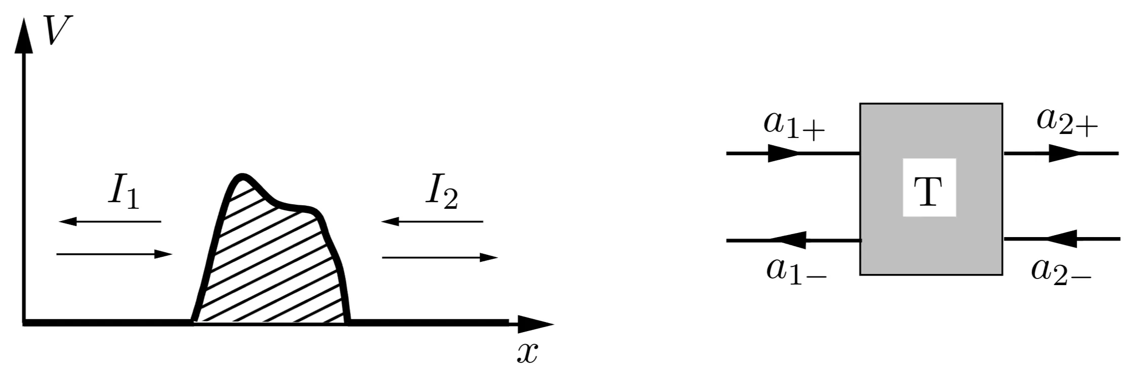
The transmission and reflection at an arbitrary potential with finite support in one dimension can be described by a transfer matrix $\hat{T}$ .

Attachments/Script 67.webp|700

In this situation, a suitable choice for a basis of the electron states is the set of plane waves ${e^{\pm i k x}}$ (see the conceptual diagram) moving in the positive (negative) $x$ -direction with wave vector $+ k$ ( $- k$ ). Only plane waves with the same $| k |$ on the left ( $I_{1}$ ) and right ( $I_{2}$ ) side of the scatterer are interconnected. Therefore, we write

\begin{aligned} ψ_{1} (x) & = a_{1 +} e^{i k x} + a_{1 -} e^{- i k x} \\ ψ_{2} (x) & = a_{2 +} e^{i k x} + a_{2 -} e^{- i k x} \end{aligned}

where $ψ_{1} (ψ_{2})$ is defined in the area $I_{1} (I_{2})$ . The vectors $a_{i} = (\begin{matrix} a_{i +} \\ a_{i -} \end{matrix})$ for $i \in {1, 2}$ are connected via the linear relation,

\begin{array}{r} a_{2} = \hat{T} a_{1} = (\begin{array}{ll} T_{11} & T_{12} \\ T_{21} & T_{22} \end{array}) a_{1}, \end{array}

with the $2 \times 2$ transfer matrix $\hat{T}$ . The conservation of current ( $J_{1} = J_{2}$ ) requires that $\hat{T}$ is unimodular, that is, $\det \hat{T} = 1$ . Here,

\begin{array}{r} J = \frac{i ℏ}{2 m} (\frac{d ψ^{*} (x)}{d x} ψ (x) - ψ^{*} (x) \frac{d ψ (x)}{d x}) \end{array}

such that, for a plane wave $ψ (x) = (1 / \sqrt{L}) e^{i k x}$ in a system of length $L$ , the current results in

\begin{array}{r} J = v / L \end{array}

with the velocity $v$ defined as $v = ℏ k / m$ . Time reversal symmetry implies that, simultaneously with $ψ (x)$ , the complex conjugate $ψ^{*} (x)$ is a solution of the stationary Schrödinger equation. From this, we find $T_{11} = T_{22}^{*}$ and $T_{12} = T_{21}^{*}$ , such that

\begin{array}{r} \hat{T} = (\begin{array}{ll} T_{11} & T_{12} \\ T_{12}^{*} & T_{11}^{*} \end{array}) . \end{array}

It is easily shown that a shift of the scattering potential by a distance $x_{0}$ changes the coefficient $T_{12}$ of $\hat{T}$ by a phase factor $e^{i 2 k x_{0}}$ . Meanwhile, the coefficient $T_{11}$ remains unchanged.
With the Ansatz for a right moving incoming wave ( $\sim e^{i k x}$ ), producing a reflected ( $\sim r e^{- i k x}$ ) and transmitted ( $\sim t e^{i k x}$ ) part, the wave functions on both sides of the scatterer read

\begin{aligned} ψ_{1} (x) & = \frac{1}{\sqrt{L}} (e^{i k x} + r e^{- i k x}) \\ ψ_{2} (x) & = \frac{1}{\sqrt{L}} (t e^{i k x}) . \end{aligned}

The coefficients of $\hat{T}$ can be determined explicitly in this situation, resulting in

\begin{array}{r} \hat{T} = (\begin{array}{cc} \frac{1}{t^{*}} & - \frac{r^{*}}{t^{*}} \\ - \frac{r}{t} & \frac{1}{t} \end{array}) . \end{array}

Here, the conservation of currents imposes the condition $1 = | r |^{2} + | t |^{2}$ . Furthermore, we can find a relation between the parameters $(r, t)$ of the potential barrier and the electric resistivity. For this, we notice that the incoming current density $J_{0}$ is split into a reflected $J_{r}$ and transmitted $J_{t}$ part, all given by

\begin{aligned} J_{0} & = - \frac{1}{L} v e = - n_{0} v e, \\ J_{r} & = - \frac{| r |^{2}}{L} v e = - n_{r} v e, \\ J_{t} & = - \frac{| t |^{2}}{L} v e = - n_{t} v e, \end{aligned}

with the velocity $v = ℏ k / m$ , the electron charge $- e$ , and the particle densities $n_{0}, n_{r}$ , and $n_{t}$ corresponding to the incoming, reflected and transmitted particles respectively. The electron density on the two sides of the barrier is given by

\begin{aligned} n_{1} & = n_{0} + n_{r} = \frac{1 + | r |^{2}}{L}, \\ n_{2} & = n_{t} = \frac{| t |^{2}}{L} . \end{aligned}

From this consideration, a density difference $δ n = n_{1} - n_{2} = (1 + | r |^{2} - | t |^{2}) / L = 2 | r |^{2} / L$ results between the left and the right side of the scatterer. The resistance $R$ of the barrier is defined by the ratio between the voltage drop over the resistor $δ V$ and the transmitted current $J_{t}$ , that is

\begin{array}{r} R = \frac{δ V}{J_{t}} . \end{array}

Consequently, a relation between $δ V$ and the electron density $δ n$ remains to be established to determine $R$ . The connection is easily found via the existing energy difference $δ E = - e δ V$ between the two sides of the resistor, such that the expression

\begin{array}{r} δ n = \frac{d n}{d E} δ E = \frac{d n}{d E} (- e δ V) \end{array}

produces the wished relation. Here, $\frac{d n}{d E} d E$ is the number of states per unit length in the energy interval $[E, E + d E]$ and we find (for spin-degenerate electrons)

\begin{aligned} \frac{d n}{d E} & = \frac{1}{L} \sum_{k, s} δ (E - \frac{ℏ^{2} k^{2}}{2 m}) \\ = 2 \int \frac{d k}{2 π} δ (E - \frac{ℏ^{2} k^{2}}{2 m}) = \frac{2}{π ℏ v (E)} . \end{aligned}

The resistance $R$ is finally obtained from the preceding relations, leading to

\begin{array}{r} R = \frac{h}{2 e^{2}} \frac{| r |^{2}}{| t |^{2}} . \end{array}

The Klitzing constant $R_{K} = h / e^{2} \approx 25.8 k Ω$ is a resistance quantum named after the discoverer of the Quantum Hall Effect. This result is the famous Landauer formula, which is valid for all one-dimensional systems and whose application often extends to the description of mesoscopic systems and quantum wires. (Note: the factor of 2 in $h / (2 e^{2})$ arises from including spin degeneracy).

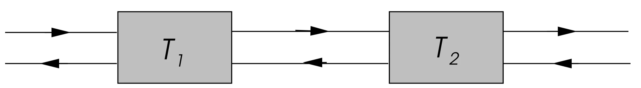
6.8.2 Scattering at Two Impurities

We consider now two spatially separated scattering potentials, represented by ${\hat{T}}_{1}$ and ${\hat{T}}_{2}$ each determined by $r_{1}, t_{1}$ and $r_{2}, t_{2}$ respectively:

Attachments/Script 68.webp|700

The particles are multiply scattered at these potentials in a unknown manner, but the global result can again be expressed via a simple transfer matrix $\hat{T} = {\hat{T}}_{1} {\hat{T}}_{2}$ , given by the matrix multiplication of each transfer matrix. All previously found properties remain valid for the new matrix $\hat{T}$ , given by

\begin{array}{r} \hat{T} = (\begin{array}{cc} \frac{1}{t_{1}^{*} t_{2}^{*}} + \frac{r_{1}^{*} r_{2}}{t_{1}^{*} t_{2}} & - \frac{r_{2}^{*}}{t_{1}^{*} t_{2}^{*}} - \frac{r_{1}^{*}}{t_{1}^{*} t_{2}} \\ - \frac{r_{1}}{t_{1} t_{2}^{*}} - \frac{r_{2}}{t_{1} t_{2}} & \frac{1}{t_{1} t_{2}} + \frac{r_{1} r_{2}^{*}}{t_{1} t_{2}^{*}} \end{array}) = (\begin{array}{cc} \frac{1}{t^{*}} & - \frac{r^{*}}{t^{*}} \\ - \frac{r}{t} & \frac{1}{t} \end{array}) . \end{array}

For the ratio between reflection and transmission probability we find

\begin{aligned} \frac{| r |^{2}}{| t |^{2}} & = \frac{1}{| t |^{2}} - 1 \\ = \frac{1}{{| t_{1} |}^{2} {| t_{2} |}^{2}} {| 1 + \frac{r_{1} r_{2}^{*} t_{2}}{t_{2}^{*}} |}^{2} - 1 \\ = \frac{1}{{| t_{1} |}^{2} {| t_{2} |}^{2}} (1 + {| r_{1} |}^{2} {| r_{2} |}^{2} + \frac{r_{1} r_{2}^{*} t_{2}}{t_{2}^{*}} + \frac{r_{1}^{*} r_{2} t_{2}^{*}}{t_{2}}) - 1. \end{aligned}

Assuming a (random) distance $d = x_{2} - x_{1}$ between the two potential barriers, we may average over this distance. Note, that for $x_{1} = 0$ , we find $r_{2} \sim e^{- 2 i k d}$ , while $r_{1}, t_{1}$ , and $t_{2}$ are independent on $d$ . Consequently, all terms containing an odd power of $r_{2}$ or $r_{2}^{*}$ vanish after averaging over $d$ . The remainders of this expression can be collected to

\begin{aligned} {\frac{| r |^{2}}{| t |^{2}} |}_{avg} & = \frac{1}{{| t_{1} |}^{2} {| t_{2} |}^{2}} (1 + {| r_{1} |}^{2} {| r_{2} |}^{2}) - 1 \\ = \frac{{| r_{1} |}^{2}}{{| t_{1} |}^{2}} + \frac{{| r_{2} |}^{2}}{{| t_{2} |}^{2}} + 2 \frac{{| r_{1} |}^{2}}{{| t_{1} |}^{2}} \frac{{| r_{2} |}^{2}}{{| t_{2} |}^{2}} . \end{aligned}

Even though two scattering potentials are added in series, an additional non-linear combination emerges beside the sum of the two ratios ${| r_{i} |}^{2} / {| t_{i} |}^{2}$ . It results from the Landauer formula applied to two scatterers, that resistances do not add linearly to the total resistance. Adding $R_{1}$ and $R_{2}$ serially, the total resistance is not given by $R = R_{1} + R_{2}$ , but by

\begin{array}{r} R = R_{1} + R_{2} + 2 \frac{R_{1} R_{2}}{R_{K}^{'}} > R_{1} + R_{2}, \end{array}

with $R_{K}^{'} = h / (2 e^{2})$ . This result is a consequence of the unavoidable multiple scattering in one dimension. This effect is particularly prominent if $R_{i} ≫ h / (2 e^{2})$ for $i \in {1, 2}$ , where resistances are then multiplied instead of summed in the interaction term.

6.8.3 Anderson Localisation

Let us consider a system with many arbitrarily distributed scatterers, and let $ρ$ be a mean resistance per unit length. $R (ℓ)$ shall be the resistance between points 0 and $ℓ$ . The change in resistance by advancing an infinitesimal $δ ℓ$ is found from the result for two scatterers, resulting in

\begin{array}{r} d R = ρ d ℓ + 2 \frac{R (ℓ)}{R_{K}^{'}} ρ d ℓ \end{array}

which yields

\begin{array}{r} \int_{0}^{ℓ} ρ d ℓ = \int_{0}^{R (ℓ)} \frac{d R}{1 + 2 R / R_{K}^{'}} \end{array}

and thus,

\begin{array}{r} ρ ℓ = \frac{R_{K}^{'}}{2} \ln (1 + 2 R (ℓ) / R_{K}^{'}) . \end{array}

Finally, solving this equation for $R (ℓ)$ , we find

\begin{array}{r} R (ℓ) = \frac{R_{K}^{'}}{2} (e^{2 ρ ℓ / R_{K}^{'}} - 1) . \end{array}

Obviously, $R$ grows almost exponentially fast for increasing $ℓ$ . This means, that for large $ℓ$ , the system is an insulator for arbitrarily small but finite $ρ > 0$ . The reason for this is that, in one dimension, all states are bound states in the presence of disorder. This phenomenon is called Anderson localisation. Even though all states are localised, the energy spectrum is continuous, as infinitely many bound states with different energy exist. The mean localisation length $ξ$ of individual states, related to the mean extension of a wave function, is found from this equation to be $ξ = R_{K}^{'} / (2 ρ)$ . The transmission amplitude is reduced on this length scale, since $| t |^{2} \approx 2 e^{- ℓ / ξ}$ for $ℓ ≫ ξ$ . In one dimension, there is no linearly increasing electric resistance. For non-interacting particles, only two extreme situations are possible. Either, the potential is perfectly periodic and the states correspond to Bloch waves. Then, coherent constructive interference produces extended states that propagate freely throughout the system, resulting in a perfect conductor without resistance. On the other hand, if the scattering potential is disordered, all states are strictly localised. In this case, there is no propagation and the system is an insulator. In three-dimensional systems, the effects of multiple scattering are far less drastic and the Ohmic law is applicable. Localisation effects in two dimensions are a very subtle topic and part of today's research in solid state physics.
We have also seen in the context of chiral edge states in the Quantum Hall state, that perfect conductance in a one-dimensional channel is obtained if there is no backscattering due to the lack of states moving in the opposite direction. In chiral states, particle move only in one direction.