Table of Contents

5.1 Lifetime of Quasi-Particles
5.2 Phenomenological Theory of Fermi Liquids
5.3 Microscopic Considerations

5 Landau's Theory of Fermi Liquids

In the previous chapters, we considered the electrons of the system as more or less independent particles. The effect of their mutual interactions only entered via the renormalisation of potentials and in the emergence of collective excitations. The underlying assumptions of our earlier discussions were that electrons in the presence of interactions can still be described as Fermionic particles with a well-defined energy-momentum relation, and that their ground state is a filled Fermi sea with a sharp Fermi surface. Since there is no guarantee that this hypothesis holds in general (and indeed, this is not always true), we have to show that in metals the description of electrons as quasi-particles is justified. This quasi-particle picture will lead us to Landau's phenomenological theory of Fermi liquids. Indeed, it is very surprising that a strongly interacting many-electron system does not end up in an extremely complex quantum state. What saves us are two important points:

In a metal the long-ranged Coulomb interaction is screened and becomes short-ranged;
The Pauli principle reduces the phase space of low-energy excitations of electrons dramatically, at least in a three-dimensional system (quantum protection).

5.1 Lifetime of Quasi-Particles

We first consider the lifetime of a state consisting of a filled Fermi sea to which one electron is added. Let $k$ with $| k | > k_{F}$ ( $ϵ_{k} = ℏ^{2} | k |^{2} / (2 m)$ with $ϵ_{k} > ϵ_{F}$ ) be the momentum (energy) of the additional electron. Due to interactions between the electrons, this state will decay into a many-body state. In momentum space such an interaction takes the form

\begin{array}{r} H_{e e} = \sum_{k, k^{'}, q} \sum_{s, s^{'}} V (q) {\hat{c}}_{k - q, s}^{†} {\hat{c}}_{k^{'} + q, s^{'}}^{†} {\hat{c}}_{k^{'}, s^{'}} {\hat{c}}_{k, s} \end{array}

where $V (q)$ represents the electron-electron interaction in momentum space while $q$ indicates the momentum transfer in the scattering process. Below, the short-ranged Yukawa potential

\begin{array}{r} V (q) = \frac{4 π e^{2}}{| q |^{2} ε (q, 0)} = \frac{4 π e^{2}}{| q |^{2} + k_{T F}^{2}} \end{array}

derived in the discussion of Thomas-Fermi screening will be used. As we are only interested in very small energy transfers $ℏ ω ≪ ϵ_{F}$ , the static approximation is admissible.
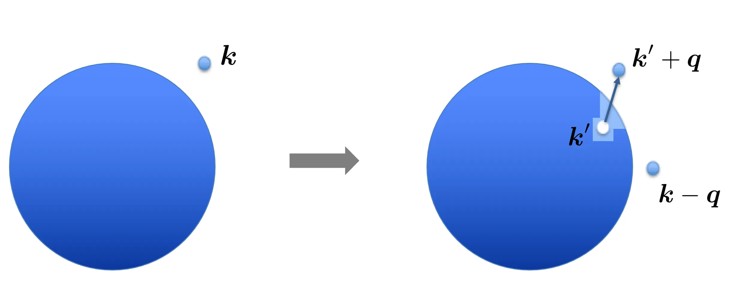
In a perturbative treatment, the lowest order effect of the interaction is the creation of a particle-hole excitation in addition to the single electron above the Fermi energy. As the additional electron changes its momentum from $k$ to $k - q$ , a hole appears at $k^{'}$ and a second electron with wavevector $k^{'} + q$ is created outside the Fermi sea. The transition is allowed whenever both energy and momentum are conserved. Momentum conservation for the process $k + k^{'} \to (k - q) + (k^{'} + q)$ is trivially satisfied. Energy conservation requires

\begin{array}{r} ϵ_{k} + ϵ_{k^{'}} = ϵ_{k - q} + ϵ_{k^{'} + q} . \end{array}

Alternatively, for the decay of the particle $k$ , its energy loss must equal the energy of the created particle-hole pair: $ϵ_{k} - ϵ_{k - q} = ϵ_{k^{'} + q} - ϵ_{k^{'}}$ .

We calculate the lifetime $τ_{k}$ of the initial state with momentum $k$ using Fermi's golden rule, yielding the transition rate from the initial state of a filled Fermi sea and one particle with momentum $k$ to a state with two electrons above the Fermi sea, with momenta $k - q$ and $k^{'} + q$ , and a hole with $k^{'}$ :

Attachments/Script 51.webp|700

Since neither the momenta $k^{'}$ and $q$ , nor the spin of the created electron are fixed, a summation over the possible configuration has to be performed, leading to

\begin{array}{r} \frac{1}{τ_{k}} = \frac{2 π}{ℏ} \frac{1}{Ω^{2}} \sum_{k^{'}, q} \sum_{s^{'}} | V (q) |^{2} n_{0, k^{'}} (1 - n_{0, k - q}) (1 - n_{0, k^{'} + q}) δ (ϵ_{k - q} + ϵ_{k^{'} + q} - ϵ_{k} - ϵ_{k^{'}}) . \end{array}

Note that the term $n_{0, k^{'}} (1 - n_{0, k - q}) (1 - n_{0, k^{'} + q})$ takes care of the Pauli principle, by ensuring that the final state after the scattering process exists, that is the hole state $k^{'}$ lies inside and the two particle states $k - q$ and $k^{'} + q$ lie outside the Fermi sea. First the integral over $k^{'}$ is performed under the condition that the energy $ϵ_{k^{'} + q} - ϵ_{k^{'}}$ of the excitation is small. With that, the integral reduces to

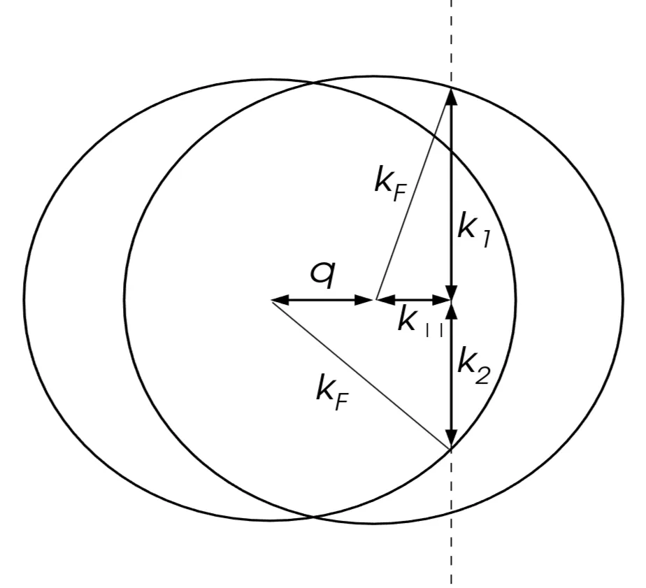
\begin{aligned} S (ω_{q, k}, q) & = \frac{1}{Ω} \sum_{k^{'}} n_{0, k^{'}} (1 - n_{0, k^{'} + q}) δ (ϵ_{k^{'} + q} - ϵ_{k^{'}} - ℏ ω_{q, k}) \\ = \frac{1}{(2 π)^{3}} \int d^{3} k^{'} n_{0, k^{'}} (1 - n_{0, k^{'} + q}) δ (ϵ_{k^{'} + q} - ϵ_{k^{'}} - ℏ ω_{q, k}) \\ = \frac{N (ϵ_{F})}{4} \frac{ω_{q, k}}{q v_{F}} \end{aligned}

where $N (ϵ_{F}) = m k_{F} / (π^{2} ℏ^{2})$ is the density of states (for one spin direction) of the electrons at the Fermi surface and $ℏ ω_{q, k} = ϵ_{k} - ϵ_{k - q} = ℏ^{2} (2 k \cdot q - | q |^{2}) / (2 m) > 0$ is the energy loss of the decaying electron. Here $q = | q |$ . Small $ω_{q, k}$ are justified, because $ℏ ω_{q, k} \leq ℏ^{2} (2 k_{F} q - q^{2}) / (2 m)$ for most allowed $ω_{q, k}$ . The integral may be computed using cylindrical coordinates, where the vector $q$ points along the axis of the cylinder. It results in

\begin{array}{r} S (q, ω) = \frac{1}{(2 π)^{2}} \int_{k_{2}}^{k_{1}} d k_{⊥}^{'} k_{⊥}^{'} \int_{0}^{k_{F}} d k_{∥}^{'} δ (\frac{ℏ^{2} q^{2}}{2 m} + \frac{ℏ^{2} q k_{∥}^{'}}{m} - ℏ ω) = \frac{m}{4 π^{2} ℏ^{2} q} (k_{1}^{2} - k_{2}^{2}) \end{array}

with $k_{1}^{2} = k_{F}^{2} - k_{∥, 0}^{2}$ and $k_{2}^{2} = k_{F}^{2} - {(k_{∥, 0} + q)}^{2}$ , where $k_{∥, 0} = (2 m ω - ℏ q^{2}) / (2 ℏ q)$ is enforced by the delta function.

Attachments/Script 52.webp|700

The wave vectors $k_{2}$ and $k_{1}$ are the upper and lower limits of integration determined from the condition $n_{0, k^{'}} (1 - n_{0, k^{'} + q}) > 0$ and can be obtained by simple geometric considerations. The previous expression for $S (ω_{q, k}, q)$ follows immediately.

In order to compute the remaining integral over $q$ , we assume that the matrix element $| V (q) |^{2}$ depends only weakly on $q$ when $| q | ≪ k_{F}$ . This is especially true when the interaction is short-ranged. In spherical coordinates, the integral reads (with $k = | k |, q = | q |$ )

\begin{aligned} \frac{1}{τ_{k}} & = \frac{2 π}{ℏ} \cdot \frac{N (ϵ_{F})}{4 v_{F} Ω} \sum_{q, s^{'}} | V (q) |^{2} \frac{ω_{q, k}}{q} \\ = \frac{N (ϵ_{F})}{(2 π)^{2} 2 ℏ v_{F}} \int d^{3} q | V (q) |^{2} \frac{ω_{q, k}}{q} \\ = \frac{N (ϵ_{F})}{(2 π) 4 m v_{F}} \int d q | V (q) |^{2} q^{2} \int_{θ_{1}}^{θ_{2}} d θ \sin θ (2 k \cos θ - q) \\ = \frac{N (ϵ_{F})}{(2 π) 4 m v_{F}} \int d q | V (q) |^{2} q^{2} {[- \frac{1}{4 k} (2 k \cos θ - q)^{2}]}_{θ_{1}}^{θ_{2}} . \end{aligned}

The restriction of the domain of integration of $θ$ follows from the two conditions $| k |^{2} \geq | k - q |^{2} \geq k_{F}^{2}$ and $| k - q |^{2} = k^{2} - 2 k q \cos θ + q^{2}$ . From the first condition, $\cos θ_{2} = q / (2 k)$ , and from the second, $\cos θ_{1} = (k^{2} - k_{F}^{2} + q^{2}) / (2 k q)$ . Thus,

\begin{aligned} \frac{1}{τ_{k}} & = \frac{N (ϵ_{F})}{(2 π) 4 m v_{F}} \int d q | V (q) |^{2} \frac{1}{4 k} {(k^{2} - k_{F}^{2})}^{2} \\ \approx \frac{N (ϵ_{F})}{(2 π) 4 v_{F}} \frac{m}{k_{F}} \frac{1}{ℏ^{4}} {(ϵ_{k} - ϵ_{F})}^{2} \int d q | V (q) |^{2} \\ = \frac{1}{8 π ℏ^{3}} \frac{N (ϵ_{F})}{v_{F}^{2}} {(ϵ_{k} - ϵ_{F})}^{2} \int d q | V (q) |^{2} . \end{aligned}

Note that convergence of the last integral over $q$ requires that the integrand does not diverge stronger than $q^{α}$ with $α < 1$ for $q \to 0$ . This condition is fulfilled for the screened Yukawa potential, but would not be for the unscreened Coulomb potential. Essentially, the result states that

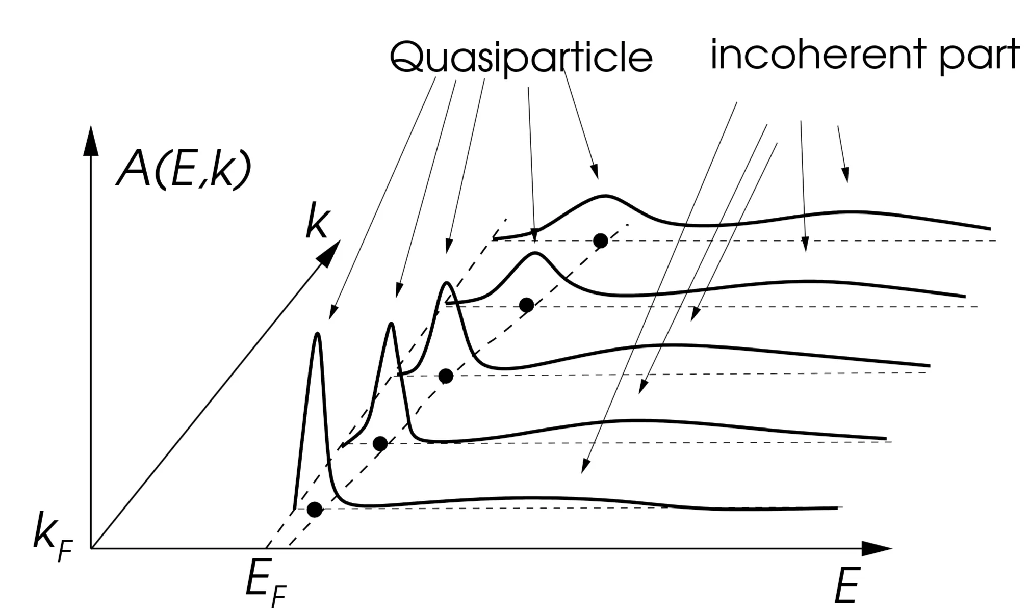
\begin{array}{r} \frac{1}{τ_{k}} \sim {(ϵ_{k} - ϵ_{F})}^{2} \end{array}

for $k$ slightly above the Fermi surface. This implies that the state $| k s ⟩$ occurs as a resonance of width $ℏ / τ_{k}$ and features a quasi-particle, which can be observed in the spectral function $A (E, k)$ as depicted here:

Attachments/Script 53.webp|700

The quasi-particle (coherent) part of the spectral function has a weight reduced from one (corresponding to the quasi-particle weight $Z_{k}$ ). The remaining weight is shifted to higher energies as a so-called incoherent part (continuum without clear momentum-energy relation). The resonance becomes arbitrarily sharp as the Fermi surface is approached

\begin{array}{r} lim_{| k | \to k_{F}} \frac{ℏ / τ_{k}}{ϵ_{k} - ϵ_{F}} = 0 \end{array}

so that the quasi-particle concept is asymptotically valid. This equation can also be seen as a verification of Heisenberg's uncertainty principle. Consequently, the momentum of an electron is a good quantum number in the vicinity of the Fermi surface. Underlying this result is the Pauli exclusion principle, which restricts the phase space for decay processes of single particle states close to the Fermi surface. In addition, the assumption of short ranged interactions is crucial. Long ranged interactions can change the behaviour drastically due to the larger number of decay channels.

5.2 Phenomenological Theory of Fermi Liquids

The existence of well-defined Fermionic quasi-particles in spite of the underlying complex many-body physics inspired Landau to formulate the following phenomenological theory. Just like the states of independent electrons, quasi-particle states shall be characterised by their momentum $k$ and spin $σ$ . In fact, there is a one-to-one mapping between the free electrons and the quasi-particles. Consequently, the number of quasi-particles and the number of electrons coincide. The momentum distribution function of quasi-particles, defined as $n_{σ} (k)$ , is subject to the condition

\begin{array}{r} N = \sum_{k, σ} n_{σ} (k) . \end{array}

In analogy to the Fermi-Dirac distribution of free electrons, one demands, that the ground state distribution function $n_{σ}^{(0)} (k)$ for the quasi-particles is described by a simple step function

\begin{array}{r} n_{σ}^{(0)} (k) = Θ (k_{F} - | k |) . \end{array}

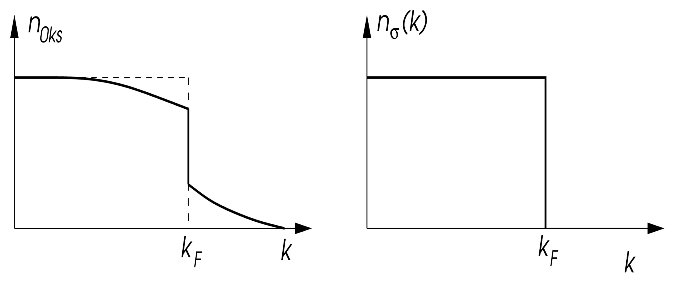
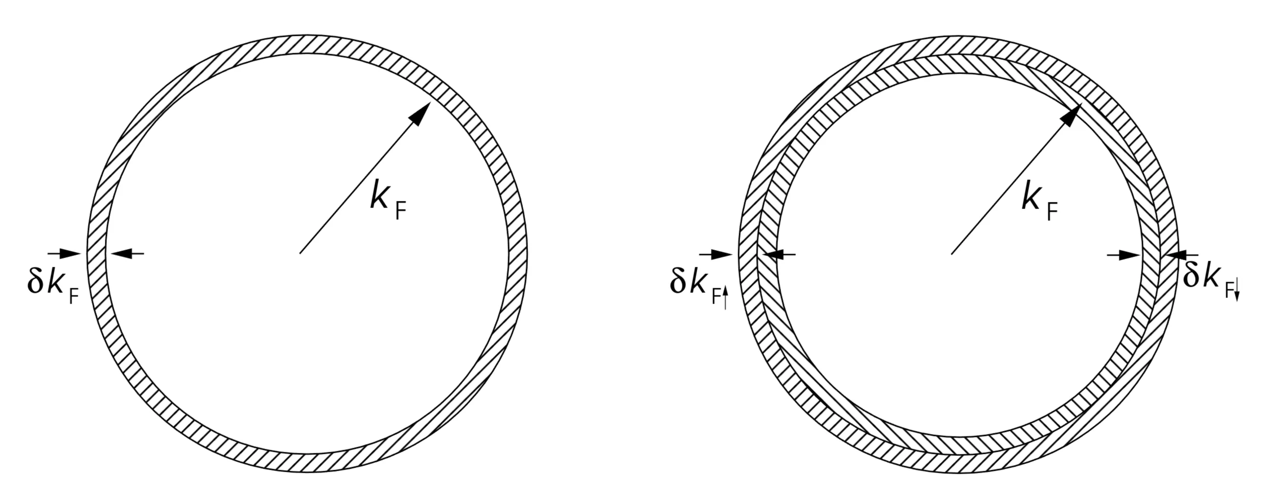
For a spherically symmetric electron system, the quasi-particle Fermi surface is a sphere with the same radius as the one for free electrons of the same density. For a general point group symmetry, the Fermi surface may be deformed by the interactions without changing the underlying symmetry. The volume enclosed by the Fermi surface is always conserved despite the deformation. Note that the distribution $n_{σ}^{(0)} (k)$ of the quasi-particles in the ground state and that $n_{0 k σ} = ⟨ {\hat{c}}_{k σ}^{†} {\hat{c}}_{k σ} ⟩$ of the real electrons in the ground state are not identical:

Attachments/Script 54.webp|700

Interestingly, $n_{0 k σ}$ is still discontinuous at the Fermi surface, but the height of the jump is, in general, smaller than unity. The modification of the electron distribution function from a step function to a "smoother" Fermi surface indicates the involvement of electron-hole excitations and the renormalisation of the electronic properties, which deplete the Fermi sea and populate the states above the Fermi level. The reduced jump in $n_{0 k σ}$ is a measure for the quasi-particle weight at the Fermi surface, $Z_{k_{F}}$ , that is, the amplitude of the corresponding free electron state in the quasi-particle state.
In Landau's theory of Fermi liquids, the essential information on the low-energy physics of the system shall be contained in the deviation of the quasi-particle distribution $n_{σ} (k)$ from its ground state distribution $n_{σ}^{(0)} (k)$ ,

\begin{array}{r} δ n_{σ} (k) = n_{σ} (k) - n_{σ}^{(0)} (k) . \end{array}

The symbol $δ$ is generally used in literature to denote this difference. Unfortunately this may suggest that the term $δ n_{σ} (k)$ is small, which is not true in general. Indeed, $δ n_{σ} (k)$ is concentrated on momenta $k$ very close to the Fermi surface only, where the quasi-particle concept is valid. This distribution function, describing the deviation from the ground state, enters a phenomenological energy functional of the form

\begin{array}{r} E = E_{0} + \sum_{k, σ} ϵ_{σ} (k) δ n_{σ} (k) + \frac{1}{2 Ω} \sum_{k, k^{'}} \sum_{σ, σ^{'}} f_{σ σ^{'}} (k, k^{'}) δ n_{σ} (k) δ n_{σ^{'}} (k^{'}) + O (δ n^{3}) \end{array}

where $E_{0}$ denotes the energy of the ground state. Moreover, the phenomenological parameters $ϵ_{σ} (k)$ and $f_{σ σ^{'}} (k, k^{'})$ have to be determined by experiments or by means of a microscopic theory. The variational derivative

\begin{array}{r} {\tilde{ϵ}}_{σ} (k) = \frac{δ E}{δ n_{σ} (k)} = ϵ_{σ} (k) + \frac{1}{Ω} \sum_{k^{'}, σ^{'}} f_{σ σ^{'}} (k, k^{'}) δ n_{σ^{'}} (k^{'}) \end{array}

yields an effective energy-momentum relation ${\tilde{ϵ}}_{σ} (k)$ , whose second term depends on the distribution of all quasi-particles. A quasi-particle moves in the "mean-field" of all other quasi-particles, so that changes $δ n_{σ} (k)$ in the distribution affect ${\tilde{ϵ}}_{σ} (k)$ . The second variational derivative describes the coupling between the quasi-particles

\begin{array}{r} \frac{δ^{2} E}{δ n_{σ} (k) δ n_{σ^{'}} (k^{'})} = \frac{1}{Ω} f_{σ σ^{'}} (k, k^{'}) . \end{array}

We introduce a parametrisation for these couplings $f_{σ σ^{'}} (k, k^{'})$ by assuming spherical symmetry of the system. Furthermore, the radial dependence is ignored, as we only consider quasi-particles in the vicinity of the Fermi surface where $| k |, | k^{'} | \approx k_{F}$ . Therefore the dependence of $f_{σ σ^{'}} (k, k^{'})$ on $k, k^{'}$ can be reduced to the relative angle $θ_{\hat{k}, {\hat{k}}^{'}}$

\begin{array}{r} f_{σ σ^{'}} (k, k^{'}) = f^{s} (\hat{k}, {\hat{k}}^{'}) + σ σ^{'} f^{a} (\hat{k}, {\hat{k}}^{'}) \end{array}

where $\hat{k} = k / | k |$ . The symmetric ( $s$ ) and antisymmetric ( $a$ ) part of $f_{σ σ^{'}} (k, k^{'})$ can be expanded in Legendre-polynomials $P_{l} (z)$ , leading to

\begin{array}{r} f^{s, a} (\hat{k}, {\hat{k}}^{'}) = \sum_{l = 0}^{\infty} f_{l}^{s, a} P_{l} (\cos θ_{\hat{k}, {\hat{k}}^{'}}) . \end{array}

The density of states at the Fermi surface is defined as (for both spins, per unit volume)

\begin{array}{r} N (ϵ_{F}) = \frac{2}{Ω} \sum_{k} δ (ϵ (k) - ϵ_{F}) = \frac{k_{F}^{2}}{π^{2} ℏ v_{F}} = \frac{m^{*} k_{F}}{π^{2} ℏ^{2}} \end{array}

and follows from the dispersion $ϵ (k)$ of the bare quasi-particle energy

\begin{array}{r} {\nabla_{k} ϵ (k) |}_{k = k_{F}} = v_{F} = \frac{ℏ k_{F}}{m^{*}} \end{array}

where for a fully rotation symmetric system we may write $ϵ (k) = ℏ^{2} | k |^{2} / (2 m^{*})$ with $m^{*}$ as an "effective mass", although we will be only interested at the spectrum in the immediate vicinity of the Fermi energy. With this definition, we also introduce the so-called Landau parameters

\begin{aligned} F_{l}^{s} & = N (ϵ_{F}) f_{l}^{s}, \\ F_{l}^{a} & = N (ϵ_{F}) f_{l}^{a}, \end{aligned}

commonly used in the literature. In the following, we want to study the relation between the different phenomenological parameters of Landau's theory of Fermi liquids and the experimentally accessible quantities of a real system, such as specific heat, compressibility, spin susceptibility among others.

5.2.1 Specific Heat - Density of States

Since the quasi-particles are Fermions, they obey Fermi-Dirac statistics

\begin{array}{r} n_{σ} (T, k) = \frac{1}{e^{[\tilde{ϵ} (k) - μ] / k_{B} T} + 1} \end{array}

with the chemical potential $μ$ , leading to

\begin{array}{r} δ n_{σ} (k) = n_{σ} (T, k) - n_{σ}^{(0)} (0, k) . \end{array}

We will only consider here the behaviour in lowest-order in temperature and restrict ourselves, therefore, to $\tilde{ϵ} (k) = ϵ (k)$ . Furthermore, we replaced $μ = ϵ_{F} + O (T^{2})$ by $ϵ_{F}$ . In order to determine the specific heat, we use the expression for the entropy of a Fermion gas based on the momentum distribution function,

\begin{array}{r} S = - \frac{k_{B}}{Ω} \sum_{k, σ} [n_{σ} (k, T) \ln (n_{σ} (k, T)) + (1 - n_{σ} (k, T)) \ln (1 - n_{σ} (k, T))] . \end{array}

Taking the derivative of the entropy $S$ with respect to $T$ , the specific heat

\begin{aligned} C (T) & = T \frac{\partial S}{\partial T} \\ = - \frac{k_{B} T}{Ω} \sum_{k, σ} \frac{e^{ξ (k) / k_{B} T}}{{(e^{ξ (k) / k_{B} T} + 1)}^{2}} \frac{ξ (k)}{k_{B} T^{2}} \ln (\frac{n_{σ} (k, T)}{1 - n_{σ} (k, T)}) \\ = \frac{k_{B} T}{Ω} \sum_{k, σ} \frac{1}{4 \cosh^{2} (ξ (k) / (2 k_{B} T))} \frac{ξ (k)}{k_{B} T^{2}} \frac{ξ (k)}{k_{B} T} \end{aligned}

is obtained, where we introduced $ξ (k) = ϵ (k) - ϵ_{F}$ . In the limit $T \to 0$ we find

\begin{aligned} \frac{C (T)}{T} & \approx \frac{N (ϵ_{F})}{4 k_{B} T^{3}} \int d ξ \frac{ξ^{2}}{\cosh^{2} (ξ / (2 k_{B} T))} \\ \approx \frac{k_{B}^{2} N (ϵ_{F})}{4} \int_{- \infty}^{+ \infty} d y \frac{y^{2}}{\cosh^{2} (y / 2)} \\ = \frac{π^{2} k_{B}^{2} N (ϵ_{F})}{3} \end{aligned}

which is the well-known linear behaviour $C (T) = γ T$ for the specific heat at low temperatures, with $γ = π^{2} k_{B}^{2} N (ϵ_{F}) / 3$ . Since $N (ϵ_{F}) = m^{*} k_{F} / (π^{2} ℏ^{2})$ (total DOS per unit volume), the effective mass $m^{*}$ of the quasi-particles can directly determined by measuring the specific heat of the system.

5.2.2 Compressibility - Landau parameter $F_{0}^{s}$

A Fermi gas has a finite compressibility because each Fermion occupies a finite amount of space due to the Pauli principle. The compressibility $κ$ is defined as

\begin{array}{r} κ = - \frac{1}{Ω} {(\frac{\partial Ω}{\partial p})}_{T, N} \end{array}

where $p$ is the uniform hydrostatic pressure. The indices $T, N$ mean, that the temperature $T$ and the particle number $N$ are kept fixed. We consider the response of the Fermi liquid upon application of uniform pressure $p$ . The shift of the bare quasi-particle energies is given by

\begin{aligned} δ ϵ_{σ} (k) & = \frac{\partial ϵ_{σ} (k)}{\partial p} δ p = \frac{\partial ϵ (k)}{\partial k} \cdot \frac{\partial k}{\partial Ω} \frac{\partial Ω}{\partial p} δ p \\ = \frac{κ^{(0)}}{3} ℏ v_{k} \cdot k δ p = γ_{k} κ^{(0)} δ p \end{aligned}

with $n = N / Ω$ . We use the fact that

\begin{aligned} k & = \frac{2 π}{L} n = \frac{2 π n}{Ω^{1 / 3}} \\ ⟹ \frac{\partial k}{\partial Ω} & = - \frac{1}{3 Ω} \frac{2 π n}{Ω^{1 / 3}} = - \frac{k}{3 Ω} \end{aligned}

and denote $γ_{k} = ℏ v_{k} \cdot k / 3 = 2 ϵ_{σ} (k) / 3$ and $κ^{(0)}$ is the unrenormalised compressibility derived below. Analogously we introduce the shift of the renormalised quasi-particle energies with the renormalised compressibility $κ$ ,

\begin{aligned} δ {\tilde{ϵ}}_{σ} (k) & = γ_{k} κ δ p = δ ϵ_{σ} (k) + \frac{1}{Ω} \sum_{k^{'}, σ^{'}} f_{σ, σ^{'}} (k, k^{'}) δ n_{σ^{'}} (k^{'}) \\ = γ_{k} κ^{(0)} δ p + \frac{1}{Ω} \sum_{k^{'}, σ^{'}} f_{σ, σ^{'}} (k, k^{'}) \frac{\partial n_{σ^{'}} (k^{'})}{\partial {\tilde{ϵ}}_{σ^{'}} (k^{'})} δ {\tilde{ϵ}}_{σ^{'}} (k^{'}) \\ = γ_{k} κ^{(0)} δ p - \frac{1}{Ω} \sum_{k^{'}, σ^{'}} f_{σ, σ^{'}} (k, k^{'}) δ ({\tilde{ϵ}}_{σ^{'}} (k^{'}) - ϵ_{F}) γ_{k^{'}} κ δ p . \end{aligned}

Changes are concentrated on the Fermi surface such that we can replace $γ_{k} \approx 2 ϵ_{F} / 3$ so that

\begin{array}{r} κ = κ^{(0)} - κ N (ϵ_{F}) \int \frac{d Ω_{{\hat{k}}^{'}}}{4 π} f^{s} (\hat{k}, {\hat{k}}^{'}) = κ^{(0)} - κ F_{0}^{s} . \end{array}

Therefore we find

\begin{array}{r} κ = \frac{κ^{(0)}}{1 + F_{0}^{s}} . \end{array}

Now we determine $κ^{(0)}$ from the volume dependence of the energy

\begin{array}{r} E^{(0)} = \sum_{k, σ} ϵ_{σ} (k) = \frac{3}{5} N ϵ_{F} = \frac{3}{5} N \frac{ℏ^{2} k_{F}^{2}}{2 m^{*}} = \frac{3}{10} \frac{ℏ^{2} N}{m^{*}} {(3 π^{2} \frac{N}{Ω})}^{2 / 3} . \end{array}

Then we determine the pressure

\begin{array}{r} p = - {(\frac{\partial E^{(0)}}{\partial Ω})}_{N} = \frac{1}{5} \frac{ℏ^{2} N}{m^{*}} {(3 π^{2} \frac{N}{Ω})}^{2 / 3} \frac{1}{Ω} \end{array}

and

\begin{array}{r} \frac{1}{κ^{(0)}} = - Ω \frac{\partial p}{\partial Ω} = \frac{1}{3} \frac{ℏ^{2} N}{m^{*} Ω} {(3 π^{2} n)}^{2 / 3} = \frac{2}{3} n ϵ_{F} . \end{array}

5.2.3 Spin Susceptibility - Landau Parameter $F_{0}^{a}$

In a magnetic field $H$ coupling to the electron spins the bare quasi-particle energy is supplemented by the Zeeman term,

\begin{array}{r} ϵ_{σ} (k) = \frac{ℏ^{2} | k |^{2}}{2 m^{*}} - g μ_{B} H \frac{σ}{2} \end{array}

where $σ = \pm 1$ denotes the spin component parallel to the applied field. The shift of the renormalised quasi-particle energy due to the applied field is

\begin{aligned} δ {\tilde{ϵ}}_{σ} (k) & = {\tilde{ϵ}}_{σ} (H, k) - \tilde{ϵ} (H = 0, k) \\ = - g μ_{B} H \frac{σ}{2} + \frac{1}{Ω} \sum_{k^{'}, σ^{'}} f_{σ, σ^{'}} (k, k^{'}) δ n_{σ^{'}} (k^{'}) \\ = - \tilde{g} μ_{B} H \frac{σ}{2} . \end{aligned}

Attachments/Script 55.webp|700

Note that by symmetry, $δ n_{σ} (k) = - δ n_{- σ} (k)$ . Due to interactions, the renormalised gyromagnetic factor $\tilde{g}$ differs from the value of $g \approx 2$ for free electrons. We focus on the second term, which can be expressed as

\begin{aligned} \frac{1}{Ω} \sum_{k^{'}, σ^{'}} f_{σ σ^{'}} (k, k^{'}) δ n_{σ^{'}} (k^{'}) & = \frac{1}{Ω} \sum_{k^{'}, σ^{'}} f_{σ σ^{'}} (k, k^{'}) \frac{\partial n_{σ^{'}}^{(0)} (k^{'})}{\partial {\tilde{ϵ}}_{σ^{'}} (k^{'})} δ {\tilde{ϵ}}_{σ^{'}} (k^{'}) \\ = \frac{1}{Ω} \sum_{k^{'}, σ^{'}} f_{σ σ^{'}} (k, k^{'}) (- δ ({\tilde{ϵ}}_{σ^{'}} (k^{'}) - ϵ_{F})) (- \tilde{g} μ_{B} H \frac{σ^{'}}{2}) . \end{aligned}

We derive

\begin{array}{r} \tilde{g} = g - \tilde{g} N (ϵ_{F}) \int \frac{d Ω_{{\hat{k}}^{'}}}{4 π} f^{a} (\hat{k}, {\hat{k}}^{'}) = g - \tilde{g} F_{0}^{a} \end{array}

or equivalently

\begin{array}{r} \tilde{g} = \frac{g}{1 + F_{0}^{a}} . \end{array}

The magnetisation of the system can be computed from the distribution function,

\begin{aligned} M & = g μ_{B} \sum_{k, σ} \frac{σ}{2} δ n_{σ} (k) = g μ_{B} \sum_{k, σ} \frac{σ}{2} \frac{\partial n_{σ}^{(0)} (k)}{\partial {\tilde{ϵ}}_{σ} (k)} δ {\tilde{ϵ}}_{σ} (k) \\ = g μ_{B} \sum_{k, σ} \frac{σ}{2} (- δ ({\tilde{ϵ}}_{σ} (k) - ϵ_{F})) (- \tilde{g} μ_{B} H \frac{σ}{2}) \end{aligned}

from which the susceptibility is immediately found to be (assuming $g \approx 2$ )

\begin{array}{r} χ = \frac{M}{H Ω} = \frac{μ_{B}^{2} N (ϵ_{F})}{1 + F_{0}^{a}} . \end{array}

The changes in the distribution function induced by the magnetic field feed back into the susceptibility, so that the latter may be either weakened ( $F_{0}^{a} > 0$ ) or enhanced ( $F_{0}^{a} < 0$ ). For the magnetic susceptibility, the Landau parameter $F_{0}^{a}$ and the effective mass $m^{*}$ (through $N (ϵ_{F})$ ) lead to a renormalisation compared to the free electron susceptibility.

5.2.4 Galilei Invariance - Effective Mass and $F_{1}^{s}$

We initially introduced by hand the effective mass of quasi-particles in $ϵ_{σ} (k)$ . In this section we show that overall consistency of the phenomenological theory requires a relation between the effective mass and one Landau parameter ( $F_{1}^{s}$ ). The reason is that the effective mass is the result of the interactions among the electrons. This self-consistency is connected with the Galilean invariance of the system. When the momenta of all particles are shifted by $ℏ q$ ( $| q |$ shall be very small compared to the Fermi momentum $k_{F}$ in order to remain within the assumption-range of the Fermi liquid theory) the distribution function given by

\begin{array}{r} δ n_{σ} (k) = n_{σ}^{(0)} (k - q) - n_{σ}^{(0)} (k) \approx - q \cdot \nabla_{k} n_{σ}^{(0)} (k) . \end{array}

This function is strongly concentrated around the Fermi energy:

Attachments/Script 56.webp|700

The current density can now be calculated, using the distribution function $n_{σ} (k) = n_{σ}^{(0)} (k) + δ n_{σ} (k)$ . Within the Fermi liquid theory this yields,

\begin{array}{r} j_{q} = \frac{1}{Ω} \sum_{k, σ} v (k) n_{σ} (k) = \frac{1}{Ω} \sum_{k, σ} v (k) δ n_{σ} (k) \end{array}

with

\begin{aligned} v (k) & = \frac{1}{ℏ} \nabla_{k} {\tilde{ϵ}}_{σ} (k) \\ = \frac{1}{ℏ} (\nabla_{k} ϵ_{σ} (k) + \frac{1}{Ω} \sum_{k^{'}, σ^{'}} \nabla_{k} f_{σ σ^{'}} (k, k^{'}) δ n_{σ^{'}} (k^{'})) . \end{aligned}

Thus we obtain for the current density,

\begin{aligned} j_{q} = & \frac{1}{Ω} \sum_{k, σ} \frac{ℏ k}{m^{*}} n_{σ} (k) + \frac{1}{Ω^{2}} \sum_{k, σ} \sum_{k^{'}, σ^{'}} [n_{σ}^{(0)} (k) + δ n_{σ} (k)] \frac{1}{ℏ} \nabla_{k} f_{σ σ^{'}} (k, k^{'}) δ n_{σ^{'}} (k^{'}) \\ = & \frac{1}{Ω} \sum_{k, σ} \frac{ℏ k}{m^{*}} δ n_{σ} (k) - \frac{1}{Ω^{2}} \sum_{k, σ} \sum_{k^{'}, σ^{'}} \frac{1}{ℏ} [\nabla_{k} n_{σ}^{(0)} (k)] f_{σ σ^{'}} (k, k^{'}) δ n_{σ^{'}} (k^{'}) + O (| q |^{2}) \\ = & \frac{1}{Ω} \sum_{k, σ} \frac{ℏ k}{m^{*}} δ n_{σ} (k) + \frac{1}{Ω^{2}} \sum_{k, σ} \sum_{k^{'}, σ^{'}} f_{σ σ^{'}} (k, k^{'}) (- δ (ϵ_{σ} (k) - ϵ_{F}) \frac{ℏ^{2} k}{m^{*}}) \\ \cdot (- q \cdot \frac{ℏ^{2} k^{'}}{m^{*}} δ (ϵ_{σ^{'}} (k^{'}) - ϵ_{F})) + O (| q |^{2}) \\ \approx & j_{1} + j_{2} . \end{aligned}

where, for the second line, we performed an integration by parts and neglect terms quadratic in $δ n$ and, in the third line, used $f_{σ σ^{'}} (k, k^{'}) = f_{σ^{'} σ} (k^{'}, k)$ and

\begin{aligned} \nabla_{k} n_{σ}^{(0)} (k) & = \frac{\partial n_{σ}^{(0)} (k)}{\partial ϵ_{σ} (k)} \nabla_{k} ϵ_{σ} (k) \\ = - δ (ϵ_{σ} (k) - ϵ_{F}) \nabla_{k} ϵ_{σ} (k) = - δ (ϵ_{σ} (k) - ϵ_{F}) \frac{ℏ^{2} k}{m^{*}} . \end{aligned}

The first term denotes quasi-particle current, $j_{1}$ , while the second term can be interpreted as a drag current, $j_{2}$ , an induced motion (backflow) of the other particles due to interactions.
From a different viewpoint, we consider the system as being in the inertial frame with a velocity $ℏ q / m$ , as all particles received the same momentum. Here $m$ is the bare electron mass. The current density is then given by

\begin{array}{r} j_{q} = \frac{N}{Ω} \frac{ℏ q}{m} = \frac{1}{Ω} \sum_{k, σ} \frac{ℏ k}{m} n_{σ} (k) = \frac{1}{Ω} \sum_{k, σ} \frac{ℏ k}{m} δ n_{σ} (k) . \end{array}

Since these two viewpoints have to be equivalent, the resulting currents should be the same. Thus, we compare the expressions for current density and obtain the equation,

\begin{array}{r} \frac{ℏ k}{m} = \frac{ℏ k}{m^{*}} + \frac{1}{Ω} \sum_{k^{'}, σ^{'}} f_{σ σ^{'}} (k, k^{'}) (- δ (ϵ_{σ^{'}} (k^{'}) - ϵ_{F}) \frac{ℏ k^{'}}{m^{*}}) \end{array}

which with $\hat{k} = k / k_{F}$ then leads to

\begin{aligned} \frac{1}{m} & = \frac{1}{m^{*}} + N (ϵ_{F}) \int \frac{d Ω_{{\hat{k}}^{'}}}{4 π} f^{s} (\hat{k}, {\hat{k}}^{'}) \frac{\hat{k} \cdot {\hat{k}}^{'}}{m^{*}} \\ = \frac{1}{m^{*}} + \frac{1}{m^{*}} \int \frac{d Ω_{{\hat{k}}^{'}}}{4 π} \underset{\sum_{l = 0}^{\infty} F_{l}^{s} P_{l} (\cos θ_{\hat{k} {\hat{k}}^{'}})}{\underset{⏟}{N (ϵ_{F}) f^{s} (\hat{k}, {\hat{k}}^{'})}} \underset{P_{1} (\cos θ_{\hat{k} {\hat{k}}^{'}})}{\underset{⏟}{\cos θ_{\hat{k} {\hat{k}}^{'}}}} \end{aligned}

or by using the orthogonality of the Legendre polynomials,

\begin{array}{r} \frac{m^{*}}{m} = 1 + \frac{1}{3} F_{1}^{s} \end{array}

where $1 / 3 = 1 / (2 l + 1)$ for $l = 1$ originates from the orthogonality relation of Legendre polynomials, as shown above. Therefore, this relation has to couple $m^{*}$ to $F_{1}^{s}$ in order for Landau's theory of Fermi liquids to be self-consistent. Generally, we find that $F_{1}^{s} > 0$ so that quasi-particles in a Fermi liquid are effectively heavier than bare electrons.

5.2.5 Stability of the Fermi Liquid

Upon inspection of the renormalisation of the quantities treated previously

\begin{aligned} \frac{γ}{γ_{0}} & = \frac{m^{*}}{m} \\ \frac{κ}{κ_{0}} & = \frac{m^{*}}{m} \frac{1}{1 + F_{0}^{s}} \\ \frac{χ}{χ_{0}} & = \frac{m^{*}}{m} \frac{1}{1 + F_{0}^{a}} \end{aligned}

with

\begin{array}{r} \frac{m^{*}}{m} = 1 + \frac{1}{3} F_{1}^{s} \end{array}

and the response functions of the non-interacting system are given by

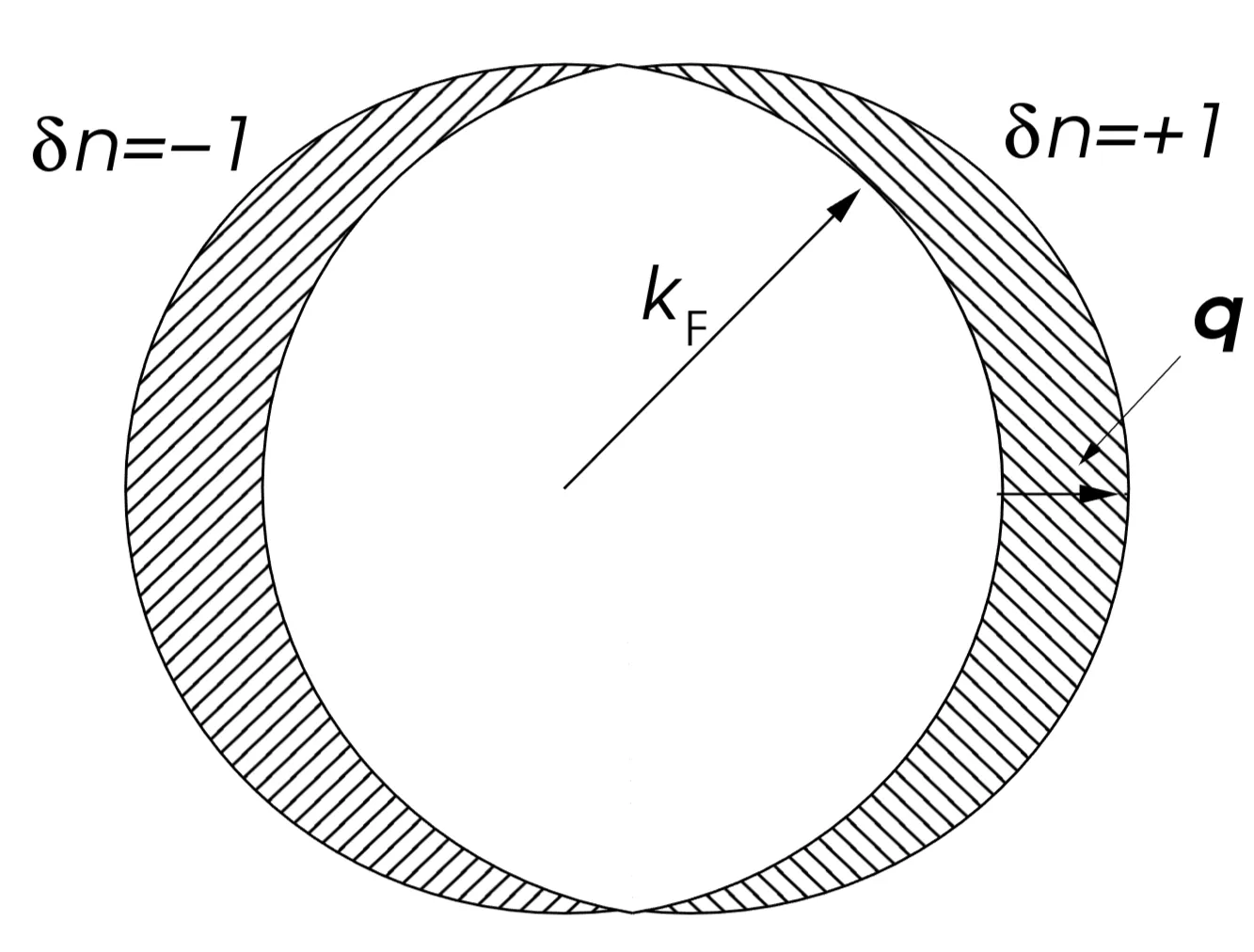
\begin{array}{r} γ_{0} = \frac{k_{B}^{2} m k_{F}}{3 ℏ^{2}}, κ_{0} = \frac{3 m}{n ℏ^{2} k_{F}^{2}} and χ_{0} = μ_{B}^{2} \frac{m k_{F}}{π^{2} ℏ^{2}} \end{array}

one notes that the compressibility $κ$ (susceptibility $χ$ ) diverges for $F_{0}^{s} \to - 1$ ( $F_{0}^{a} \to - 1$ ), indicating an instability of the system. A diverging spin susceptibility, for example, leads to a ferromagnetic state with a split Fermi surface, one for each spin direction. On the other hand, a diverging compressibility leads to a spontaneous contraction of the system. More generally, the deformation of the quasi-particle distribution function may vary over the Fermi surface, so that arbitrary deviations of the Fermi liquid ground state may be classified by the deformation

\begin{array}{r} δ n_{σ} (\hat{k}) = \sum_{l = 0}^{\infty} \sum_{m = - l}^{+ l} δ n_{σ, l, m} Y_{l m} (θ_{k}, ϕ_{k}) . \end{array}

Note that we allow here formally for complex distribution functions. For pure charge density deformations we have $δ n_{+, l, m} (\hat{k}) = δ n_{-, l, m} (\hat{k})$ , while pure spin density deformations are described by $δ n_{+, l, m} (\hat{k}) = - δ n_{-, l, m} (\hat{k})$ . The general response function for a redistribution $δ n_{σ} (\hat{k})$ with the anisotropy $Y_{l m} (θ_{k}, ϕ_{k})$ is given by

\begin{array}{r} χ_{l, m} = \frac{χ_{l, m}^{(0)}}{1 + \frac{F_{l}^{s, a}}{2 l + 1}} . \end{array}

This comes from here:
General response and distribution deformations: We consider a force field $F$ with conjugate "polarisation" $P$ which yields a modification of the quasi-particle dispersion,

\begin{array}{r} δ ϵ_{σ} (k) = - α λ_{σ} (k) F and δ {\tilde{ϵ}}_{σ} (k) = - \tilde{α} λ_{σ} (k) F \end{array}

where we assume that $λ_{σ} (k) = Y_{l, m} (θ_{\hat{k}}, ϕ_{\hat{k}}) = (- 1)^{m} Y_{l, - m}^{*} (θ_{\hat{k}}, ϕ_{\hat{k}})$ without spin dependence. Then we can write

\begin{aligned} δ {\tilde{ϵ}}_{σ} (k) & = δ ϵ_{σ} (k) + \frac{1}{Ω} \sum_{k^{'}, σ^{'}} f_{σ σ^{'}} (\hat{k}, {\hat{k}}^{'}) δ n_{σ^{'}} (k^{'}) \\ = δ ϵ_{σ} (k) + \frac{1}{Ω} \sum_{k^{'}, σ^{'}} f_{σ σ^{'}} (\hat{k}, {\hat{k}}^{'}) \frac{\partial n_{σ^{'}}}{\partial {\tilde{ϵ}}_{σ^{'}} (k^{'})} δ {\tilde{ϵ}}_{σ^{'}} (k^{'}) . \end{aligned}

In the last step we take for $δ n_{σ^{'}} (k^{'})$ the self-consistent value taking the feedback of the quasi-particle coupling into account. We now use the relation

\begin{aligned} f^{s, a} (\hat{k}, {\hat{k}}^{'}) & = \sum_{l^{'} = 0}^{\infty} f_{l^{'}}^{s, a} P_{l^{'}} (\hat{k} \cdot {\hat{k}}^{'}) \\ = 4 π \sum_{l^{'} = 0}^{\infty} \frac{f_{l^{'}}^{s, a}}{2 l^{'} + 1} \sum_{m^{'} = - l^{'}}^{+ l^{'}} Y_{l^{'} m^{'}} (θ_{\hat{k}}, ϕ_{\hat{k}}) Y_{l^{'} m^{'}}^{*} (θ_{{\hat{k}}^{'}}, ϕ_{{\hat{k}}^{'}}) \end{aligned}

and find,

\begin{array}{r} \tilde{α} λ_{σ} (k) F = α λ_{σ} (k) F - N (ϵ_{F}) \sum_{l^{'} = 0}^{\infty} \frac{f_{l^{'}}^{s}}{2 l^{'} + 1} \sum_{m^{'} = - l^{'}}^{+ l^{'}} Y_{l^{'} m^{'}} (θ_{\hat{k}}, ϕ_{\hat{k}}) \tilde{α} \underset{δ_{l l^{'}} δ_{m m^{'}}}{\underset{⏟}{\int d Ω_{{\hat{k}}^{'}} Y_{l^{'} m^{'}}^{*} (θ_{{\hat{k}}^{'}}, ϕ_{{\hat{k}}^{'}}) λ_{σ} (k^{'})}} F \end{array}

which leads straightforwardly to

\begin{array}{r} \tilde{α} = α - \tilde{α} \frac{F_{l}^{s}}{2 l + 1} ⟹ \tilde{α} = \frac{α}{1 + \frac{F_{l}^{s}}{2 l + 1}} . \end{array}

Now the polarisation is calculated which we may define as

\begin{aligned} P & = \frac{1}{Ω} \sum_{k, σ} α λ_{σ} (k)^{*} δ n_{σ} (k) = \frac{1}{Ω} \sum_{k, σ} α λ_{σ} (k)^{*} \frac{\partial n_{σ}}{\partial {\tilde{ϵ}}_{σ} (k)} δ {\tilde{ϵ}}_{σ} (k) \\ = \frac{1}{Ω} \sum_{k, σ} α (- δ (ϵ_{σ} (k) - ϵ_{F})) (- \tilde{α} | λ (k) |^{2} F) \\ = α \tilde{α} N (ϵ_{F}) F \int \frac{d Ω_{k}}{4 π} | λ (k) |^{2} = \frac{α \tilde{α} N (ϵ_{F}) F}{4 π} \end{aligned}

such that the linear response is given by

\begin{array}{r} χ = \frac{P}{F} = \frac{α^{2} N (ϵ_{F})}{4 π (1 + \frac{F_{l}^{s}}{2 l + 1})} . \end{array}

Stability of the Fermi liquid against any of these deformations requires

\begin{array}{r} 1 + \frac{F_{l}^{s, a}}{2 l + 1} > 0. \end{array}

If for any deformation channel $l$ this conditions is violated one talks about a "Pomeranchuk instability".Generally, the renormalisation of the Fermi liquid leads to a change in the Wilson ratio, defined as

\begin{array}{r} \frac{R}{R_{0}} = \frac{χ / χ_{0}}{γ / γ_{0}} = \frac{1 + F_{1}^{s} / 3}{1 + F_{0}^{a}} \end{array}

where $R_{0} = χ_{0} / γ_{0} = (g / 2)^{2} \cdot 3 μ_{B}^{2} / (π^{2} k_{B}^{2})$ . Note that the Wilson ratio does not depend on the effective mass $m^{*} / m$ directly through $F_{1}^{s}$ in this form, but rather through the $χ_{0}$ and $γ_{0}$ if $m^{*}$ is considered part of the "bare" parameters for them.
A remarkable feature of the Fermi liquid theory is that even very strongly interacting Fermions remain Fermi liquids, notably the quantum liquid $^{3} He$ and so-called heavy Fermion systems, which are compounds of transition metals and rare earths. Both are strongly renormalised Fermi liquids. For $^{3} He$ we give some of the parameters in Table 5.1 both for zero pressure and for pressures just below the critical pressure at which He solidifies ( $p_{c} \approx 2.5 MPa = 25 bar$ ).

Pressure	$m^{*} / m$	$F_{0}^{s}$	$F_{0}^{a}$	$F_{1}^{s}$	$κ / κ_{0}$	$χ / χ_{0}$
$p = 0$	3.0	10.1	-0.52	6.0	0.27	6.3
$p < p_{c}$	6.2	94	-0.74	15.7	0.065	24

The trends show obviously, that the higher the applied pressure is, the denser the liquid becomes and the stronger the quasi-particles interact. Approaching the solidification the compressibility is reduced, the quasi-particles become heavier (slower) and the magnetic response increases drastically. Finally the heavy Fermion systems are characterised by the extraordinary enhancements of the effective mass which for many of these compounds lie between 100 and 1000 times higher than the bare electron mass (for example ${CeAl}_{3}, {UBe}_{13}$ ). This large masses lead the notion of almost localised Fermi liquids, since the large effective mass is induced by the hybridisation of itinerant conduction electrons with strongly interacting (localised) electron states in partially filled $4 f$ - or $5 f$ -orbitals of Lanthanide and Actinide atoms, respectively.

5.3 Microscopic Considerations

A rigorous derivation of Landau's Fermi liquid theory requires methods of quantum field theory and would go beyond the scope of these lectures. However, plain Rayleigh-Schrödinger theory applied to a simple model allows to gain some insights into the microscopic fundament of this phenomenological theory. In the following, we consider a model of Fermions with contact interaction $U δ (r - r^{'})$ , described by the Hamiltonian

\begin{aligned} H & = \sum_{k, s} ϵ_{k} {\hat{c}}_{k s}^{†} {\hat{c}}_{k s} + \int d^{3} r d^{3} r^{'} {\hat{Ψ}}_{↑} (r)^{†} {\hat{Ψ}}_{↓} {(r^{'})}^{†} U δ (r - r^{'}) {\hat{Ψ}}_{↓} (r^{'}) {\hat{Ψ}}_{↑} (r) \\ = \sum_{k, s} ϵ_{k} {\hat{c}}_{k s}^{†} {\hat{c}}_{k s} + \frac{U}{Ω} \sum_{k, k^{'}, q} {\hat{c}}_{k + q ↑}^{†} {\hat{c}}_{k^{'} - q ↓}^{†} {\hat{c}}_{k^{'} ↓} {\hat{c}}_{k ↑} \end{aligned}

where $ϵ_{k} = ℏ^{2} | k |^{2} / (2 m)$ is a parabolic dispersion of non-interacting electrons. We previously noticed that, in order to find well-defined quasi-particles, the interaction between the Fermions has to be short-ranged. This specially holds for the contact interaction.

5.3.1 Landau Parameters

Starting from the previously defined Hamiltonian, we will determine Landau parameters for a corresponding Fermi liquid theory. For a given momentum distribution $n_{k s} = ⟨ {\hat{c}}_{k s}^{†} {\hat{c}}_{k s} ⟩ = n_{k s}^{(0)} + δ n_{k s}$ , we can expand the energy resulting from the Hamiltonian following the Rayleigh-Schrödinger perturbation method,

\begin{array}{r} E = E^{(0)} + E^{(1)} + E^{(2)} + \dots \end{array}

with

\begin{aligned} E^{(0)} & = \sum_{k, s} ϵ_{k} n_{k s}, \\ E^{(1)} & = \frac{U}{Ω} \sum_{k, k^{'}} n_{k ↑} n_{k^{'} ↓}, \\ E^{(2)} & = \frac{U^{2}}{Ω^{2}} \sum_{k, k^{'}, q} \frac{n_{k ↑} n_{k^{'} ↓} (1 - n_{k + q ↑}) (1 - n_{k^{'} - q ↓})}{ϵ_{k} + ϵ_{k^{'}} - ϵ_{k + q} - ϵ_{k^{'} - q}} . \end{aligned}

The second order term $E^{(2)}$ describes virtual processes corresponding to a pair of particle-hole excitations. The numerator of this term can be split into four different contributions.
We first consider the term quadratic in $n_{k}$ and combine it with the first order term $E^{(1)}$ , which has the same structure,

\begin{array}{r} {\tilde{E}}^{(1)} = E^{(1)} + \frac{U^{2}}{Ω^{2}} \sum_{k, k^{'}, q} \frac{n_{k ↑} n_{k^{'} ↓}}{ϵ_{k} + ϵ_{k^{'}} - ϵ_{k + q} - ϵ_{k^{'} - q}} \approx \frac{\tilde{U}}{Ω} \sum_{k, k^{'}} n_{k ↑} n_{k^{'} ↓} . \end{array}

In the last step, we defined the renormalised interaction $\tilde{U}$ through,

\begin{array}{r} \tilde{U} = U + \frac{U^{2}}{Ω} \sum_{q} \frac{1}{ϵ_{k} + ϵ_{k^{'}} - ϵ_{k + q} - ϵ_{k^{'} - q}} . \end{array}

In principle, $\tilde{U}$ depends on the wave vectors $k$ and $k^{'}$ . However, when the wave vectors are restricted to the Fermi surface ( $| k | = | k^{'} | = k_{F}$ ), and if the range of the interaction $ℓ$ is small compared to the mean electron spacing, that is, $k_{F} ℓ ≪ 1,$ this dependency may be neglected.
We should be careful with our choice of a contact interaction, since it would lead to a divergence in the large- $q$ range. A cutoff for $q$ of order $Q_{c} \sim ℓ^{- 1}$ would regularise the integral which is dominated by the large- $q$ part. Thus we may use the following expansion (with $q = | q |$ ),

\begin{aligned} \frac{1}{Ω} \sum_{q} \frac{1}{ϵ_{k} + ϵ_{k^{'}} - ϵ_{k + q} - ϵ_{k^{'} - q}} & = \frac{1}{(2 π)^{3} ℏ^{2}} \int_{0}^{Q_{c}} d q q^{2} \int d Ω_{q} \frac{m}{(k^{'} - k) \cdot q - | q |^{2}} \\ = \frac{m}{(2 π)^{2} ℏ^{2}} \int_{0}^{Q_{c}} d q q \int_{- 1}^{+ 1} \frac{d \cos θ}{K \cos θ - q} \\ = \frac{m}{(2 π)^{2} ℏ^{2}} \int_{0}^{Q_{c}} d q q \frac{1}{K} \ln | \frac{q - K}{q + K} | \\ = - \frac{m}{(2 π)^{2} ℏ^{2}} (Q_{c} + \frac{K^{2} - Q_{c}^{2}}{2 K} \ln | \frac{Q_{c} - K}{Q_{c} + K} |) \\ \approx - \frac{m Q_{c}}{(2 π)^{2} ℏ^{2}} (1 - \frac{K^{2}}{2 Q_{c}^{2}} + O (\frac{K^{4}}{Q_{c}^{4}})) \\ = - N (ϵ_{F}) \frac{Q_{c}}{2 k_{F}} \frac{π^{2} ℏ^{2}}{m k_{F}} \frac{m Q_{c}}{(2 π)^{2} ℏ^{2}} \dots \approx - N (ϵ_{F}) \frac{π Q_{c}}{4 k_{F}^{2}} \end{aligned}

where we use $K = | k^{'} - k | \leq 2 k_{F} ≪ Q_{c}$ . From this we conclude that the momentum dependence of $\tilde{U}$ is indeed weak.
Since the term quartic in $n_{k}$ vanishes due to symmetry, the remaining contribution to $E^{(2)}$ is cubic in $n_{k}$ and reads

\begin{array}{r} {\tilde{E}}^{(2)} = - \frac{{\tilde{U}}^{2}}{Ω^{2}} \sum_{k, k^{'}, q} \frac{n_{k ↑} n_{k^{'} ↓} (n_{k + q ↑} + n_{k^{'} - q ↓})}{ϵ_{k} + ϵ_{k^{'}} - ϵ_{k + q} - ϵ_{k^{'} - q}} . \end{array}

We replaced $U^{2}$ by ${\tilde{U}}^{2}$ , which is admissible at this order of the perturbative expansion. The variation of the energy $E$ with respect to $δ n_{k ↑}$ can easily be calculated,

\begin{array}{r} {\tilde{ϵ}}_{↑} (k) = ϵ_{k} + \frac{\tilde{U}}{Ω} \sum_{k^{'}} n_{k^{'} ↓} - \frac{{\tilde{U}}^{2}}{Ω^{2}} \sum_{k^{'}, q} \frac{n_{k^{'} ↓} (n_{k + q ↑} + n_{k^{'} - q ↓}) - n_{k + q ↑} n_{k^{'} - q ↓}}{ϵ_{k} + ϵ_{k^{'}} - ϵ_{k + q} - ϵ_{k^{'} - q}}, \end{array}

and an analogous expression is found for $ϵ_{↓} (k)$ . The coupling parameters $f_{σ σ^{'}} (k, k^{'})$ may be determined using the definition $f_{σ σ^{'}} = Ω \frac{δ^{2} E}{δ n_{σ} δ n_{σ^{'}}}$ . Starting with $f_{↑↑} (k_{F}, k_{F}^{'})$ with wave-vectors on the Fermi surface $(| k_{F} | = | k_{F}^{'} | = k_{F})$ , the terms contributing to the coupling can be written as

\begin{array}{r} \begin{aligned} \frac{{\tilde{U}}^{2}}{Ω^{2}} \sum_{k^{'}, q} n_{k + q ↑} \frac{n_{k^{'} - q ↓} - n_{k^{'} ↓}}{ϵ_{k} + ϵ_{k^{'}} - ϵ_{k + q} - ϵ_{k^{'} - q}} \\ \overset{k + q \to k_{F}^{'}}{⟶} & \frac{1}{Ω} \sum_{k_{F}^{'}} n_{k_{F}^{'} ↑} \frac{{\tilde{U}}^{2}}{Ω} {\sum_{k^{'}} \frac{n_{k^{'} - q ↓}^{(0)} - n_{k^{'} ↓}^{(0)}}{ϵ_{k^{'}} - ϵ_{k^{'} - q}} |}_{q = k_{F}^{'} - k_{F}} \\ = - \frac{1}{Ω} \sum_{k_{F}^{'}} n_{k_{F}^{'} ↑} \frac{{\tilde{U}}^{2}}{2} χ_{0} (k_{F}^{'} - k_{F}), \end{aligned} \end{array}

where we consider $n_{k_{F}^{'} ↑} = n_{k_{F}^{'} ↑}^{(0)} + δ n_{k_{F}^{'} ↑}$ . Note that the part in this term which depends on $n_{k_{F}^{'} ↑}^{(0)}$ will contribute the ground state energy in Landau's energy functional. Here, $χ_{0} (q)$ is the static Lindhard susceptibility. With the help of the definition $f_{σ σ^{'}} = Ω \frac{δ^{2} E}{δ n_{σ} δ n_{σ^{'}}}$ , it follows immediately, that

\begin{array}{r} f_{↑↑} (k_{F}, k_{F}^{'}) = f_{↓↓} (k_{F}, k_{F}^{'}) = \frac{{\tilde{U}}^{2}}{2} χ_{0} (k_{F} - k_{F}^{'}) . \end{array}

The other couplings are obtained in a similar way, resulting in

\begin{aligned} f_{↑↓} (k_{F}, k_{F}^{'}) & = f_{↓↑} (k_{F}, k_{F}^{'}) \\ = \tilde{U} - \frac{{\tilde{U}}^{2}}{2} [2 {\tilde{χ}}_{0} (k_{F} + k_{F}^{'}) - χ_{0} (k_{F} - k_{F}^{'})], \end{aligned}

where the function ${\tilde{χ}}_{0} (q)$ is defined as

\begin{array}{r} {\tilde{χ}}_{0} (q) = \frac{1}{Ω} \sum_{k^{'}} \frac{n_{k^{'} + q ↑}^{(0)} + n_{k^{'} ↓}^{(0)}}{2 ϵ_{F} - ϵ_{k^{'} + q} - ϵ_{k^{'}}} . \end{array}

If the couplings are parameterised by the angle $θ$ between $k_{F}$ and $k_{F}^{'}$ , they can be expressed as

\begin{aligned} f_{σ σ^{'}} (θ) = \frac{\tilde{U}}{2} & [(1 + \frac{\tilde{U} N (ϵ_{F})}{4} (2 + \frac{\cos θ}{2 \sin (θ / 2)} \ln \frac{1 + \sin (θ / 2)}{1 - \sin (θ / 2)})) δ_{σ - σ^{'}} \\ - (1 + \frac{\tilde{U} N (ϵ_{F})}{4} (1 - \frac{\sin (θ / 2)}{2} \ln \frac{1 + \sin (θ / 2)}{1 - \sin (θ / 2)})) (1 - δ_{σ - σ^{'}})] . \end{aligned}

Finally, we are in the position to determine the most important Landau parameters by matching these expressions to the parametrisation,

\begin{aligned} F_{0}^{s} & = \tilde{u} [1 + \tilde{u} (1 + \frac{1}{6} (2 + \ln 2))] \\ F_{0}^{a} & = - \tilde{u} [1 + \tilde{u} (1 - \frac{2}{3} (1 - \ln 2))] \\ F_{1}^{s} & = {\tilde{u}}^{2} \frac{2}{15} (7 \ln 2 - 1) \end{aligned}

where $\tilde{u} = \tilde{U} N (ϵ_{F}) / 2$ has been introduced for better readability. Since the Landau parameter $F_{1}^{s}$ is responsible for the modification of the effective mass $m^{*}$ compared to the bare mass $m$ , $m^{*}$ is enhanced compared to $m$ for both attractive $(U < 0)$ and repulsive $(U > 0)$ interactions. Obviously, the sign of the interaction $U$ does not affect the renormalisation of the effective mass $m^{*}$ . This is so, because the existence of an interaction (whatever sign it has) between the particles enforces the motion of many particles whenever one is moved. The behaviour of the susceptibility and the compressibility depends on the sign of the interaction. If the interaction is repulsive $(\tilde{u} > 0)$ , the compressibility decreases $(F_{0}^{s} > 0)$ , implying that it is harder to compress the Fermi liquid. The susceptibility is enhanced $(F_{0}^{a} < 0)$ in this case, so that it is easier to polarise the spins of the electrons. Conversely, for attractive interactions ( $\tilde{u} < 0$ ), the compressibility is enhanced due to a negative Landau parameter $F_{0}^{s}$ , whereas the susceptibility is suppressed with a factor $1 / (1 + F_{0}^{a})$ , with $F_{0}^{a} > 0$ . The attractive case is more subtle because the Fermi liquid becomes unstable at low temperatures, turning into a superfluid or superconductor, by forming so-called Cooper pairs. This represents another non-trivial Fermi surface instability.

5.3.2 Distribution Function

Finally, we examine the effect of interactions on the ground state properties, using again Rayleigh-Schrödinger perturbation theory. The calculation of the corrections to the ground state $| Ψ_{0} ⟩$ , the filled Fermi sea can be expressed as

\begin{array}{r} | Ψ ⟩ = | Ψ^{(0)} ⟩ + | Ψ^{(1)} ⟩ + \dots \end{array}

where

\begin{aligned} | Ψ^{(0)} ⟩ & = | Ψ_{0} ⟩ \\ | Ψ^{(1)} ⟩ & = \frac{U}{Ω} \sum_{k, k^{'}, q} \sum_{s, s^{'}} \frac{{\hat{c}}_{k + q, s}^{†} {\hat{c}}_{k^{'} - q, s^{'}}^{†} {\hat{c}}_{k^{'}, s^{'}} {\hat{c}}_{k, s}}{ϵ_{k} + ϵ_{k^{'}} - ϵ_{k + q} - ϵ_{k^{'} - q}} | Ψ_{0} ⟩ . \end{aligned}

The state $| Ψ_{0} ⟩$ represents the ground state of non-interacting Fermions. The lowest order correction involves particle-hole excitations, depleting the Fermi sea by lifting particles virtually above the Fermi energy. How this correction affects the distribution function, will be discussed next. The momentum distribution $n_{k s} = ⟨ {\hat{c}}_{k s}^{†} {\hat{c}}_{k s} ⟩$ is obtain as the expectation value,

\begin{array}{r} n_{k s} = \frac{⟨ Ψ | {\hat{c}}_{k s}^{†} {\hat{c}}_{k s} | Ψ ⟩}{⟨ Ψ ∣ Ψ ⟩} = n_{k s}^{(0)} + δ n_{k s}^{(2)} + \dots \end{array}

where $n_{k s}^{(0)}$ is the unperturbed distribution $Θ (k_{F} - | k |)$ , and

\begin{array}{r} δ n_{k s}^{(2)} = {\begin{cases} - \frac{U^{2}}{Ω^{2}} \sum_{k_{1}, k_{2}, k_{3}} \frac{(1 - n_{k_{1}}) (1 - n_{k_{2}}) n_{k_{3}}}{{(ϵ_{k} + ϵ_{k_{3}} - ϵ_{k_{1}} - ϵ_{k_{2}})}^{2}} δ_{k + k_{3}, k_{1} + k_{2}} & | k | < k_{F} \\ \frac{U^{2}}{Ω^{2}} \sum_{k_{1}, k_{2}, k_{3}} \frac{n_{k_{1}} n_{k_{2}} (1 - n_{k_{3}})}{{(ϵ_{k_{1}} + ϵ_{k_{2}} - ϵ_{k} - ϵ_{k_{3}})}^{2}} δ_{k + k_{3}, k_{1} + k_{2}} & | k | > k_{F} \end{cases} . \end{array}

This yields the modification of the distribution functions as shown here:

Attachments/Script 57.webp|700

It allows us also to determine the size of the discontinuity of the distribution function at the Fermi surface,

\begin{array}{r} n_{k_{F}^{-}} - n_{k_{F}^{+}} = 1 - {(\frac{U N (ϵ_{F})}{2})}^{2} \ln (2), \end{array}

where

\begin{array}{r} n_{k_{F}^{\pm}} = lim_{| k | - k_{F} \to 0^{\pm}} (n_{k}^{(0)} + δ n_{k}^{(2)}) . \end{array}

The jump of $n_{k}$ at the Fermi surface is reduced independently of the sign of the interaction. The reduction is quadratic in the perturbation parameter $U N (ϵ_{F})$ . This jump is also a measure for the weight of the quasi-particle state at the Fermi surface.

5.3.3 Fermi Liquid in One Dimension?

Within a perturbative approach the Fermi liquid theory can be justified for a three-dimensional system, and we recognise the one-to-one correspondence between bare electrons and quasi-particles renormalised by (short-ranged) interactions. Now we would like to show that within the same approach problems appear in one-dimensional systems, which are of a conceptual nature and hint that interacting Fermions in one dimension would not form a Fermi liquid, but a Luttinger liquid, as we will motivate briefly below.
The Landau parameters have been expressed above in terms of the response functions $χ_{0} (q = k_{F} - k_{F}^{'})$ and ${\tilde{χ}}_{0} (q = k_{F} - k_{F}^{'})$ . For the one-dimensional system, the relevant contributions come from two configurations, since there are two Fermi points only (instead of a two-dimensional Fermi surface),

\begin{array}{r} (k_{F}, k_{F}^{'}) \Rightarrow q = k_{F} - k_{F}^{'} = 0, \pm 2 k_{F} . \end{array}

We find that the response functions show singularities for some of these momenta, and we obtain

\begin{array}{r} f_{↑↑} (\pm k_{F}, \pm k_{F}) = f_{↓↓} (\pm k_{F}, \mp k_{F}) \to \infty \end{array}

as well as

\begin{array}{r} f_{↑↓} (k_{F}, \pm k_{F}) = f_{↓↑} (k_{F}, \mp k_{F}) \to \infty \end{array}

giving rise to the divergence of all Landau parameters. Therefore the perturbative approach to a Landau Fermi liquid is not allowed for the one-dimensional Fermi system.

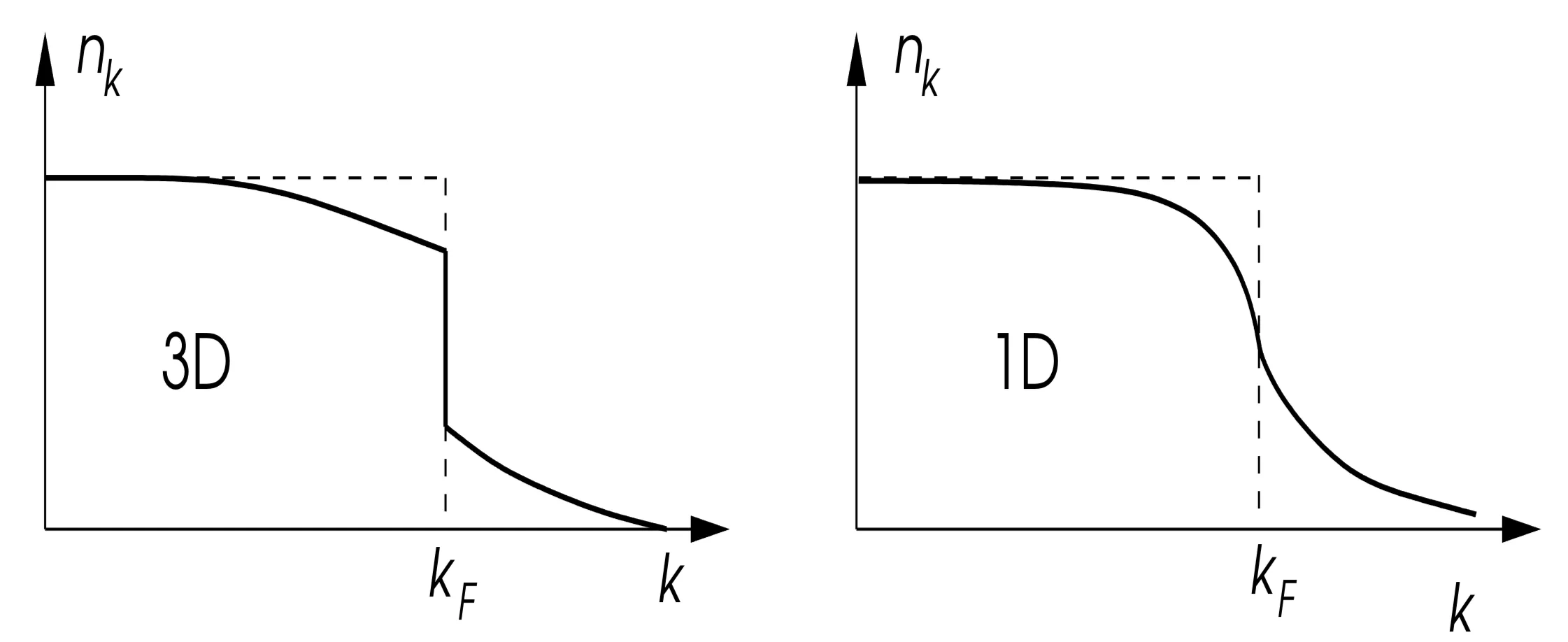
The same message is obtained when looking at the momentum distribution form which had in three dimensions a step giving a measure for the (reduced but finite) quasi-particle weight. The analogous calculation as in the previous subsection leads here to (for scalar $k$ in 1D)

\begin{array}{r} n_{k s}^{(2)} \approx {\begin{cases} \frac{1}{8 π^{2}} \frac{U^{2}}{ℏ^{2} v_{F}^{2}} \ln \frac{k_{+}}{k - k_{F}} & k > k_{F} \\ - \frac{1}{8 π^{2}} \frac{U^{2}}{ℏ^{2} v_{F}^{2}} \ln \frac{k_{-}}{k_{F} - k} & k < k_{F} \end{cases} . \end{array}

Here, $k_{\pm}$ are cutoff parameters of the order of the Fermi wave vector $k_{F}$ . Apparently the quality of the perturbative calculation deteriorates as $k \to k_{F \pm}$ , since we encounter a logarithmic divergence from both sides.

Attachments/Script 58.webp|700

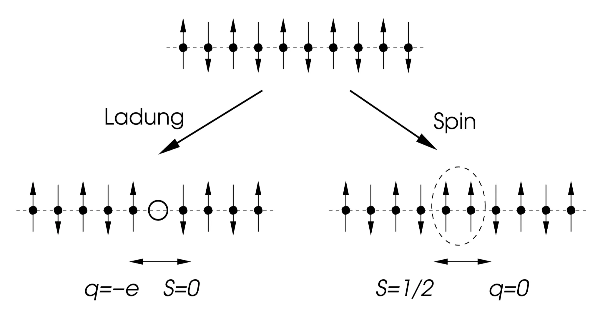
Indeed, a more elaborated approach shows that the distribution function is continuous at $k = k_{F}$ in one dimension, without any jump. Correspondingly, the quasi-particle weight vanishes and the elementary excitations cannot be described by Fermionic quasi-particles but rather by collective modes. Landau's Theory of Fermi liquids is inappropriate for such systems. This kind of behaviour, where the quasi-particle weight vanishes, can be described by the so-called bosonisation of Fermions in one dimension, a topic that is beyond the scope of these lectures. However, a result worth mentioning, shows that the Fermionic excitations in one dimensions decay into independent charge and spin excitations, the so-called spin-charge separation. This behaviour can be understood with the naive picture of a half-filled lattice with predominantly antiferromagnetic spin correlations. In this case both charge excitations (empty or doubly occupied lattice site) and spin excitations (two parallel neighbouring spins) represent different kinds of domain walls, and are free to move at different velocities.

5 Landau's Theory of Fermi Liquids

5.1 Lifetime of Quasi-Particles

5.2 Phenomenological Theory of Fermi Liquids

5.2.1 Specific Heat - Density of States

5.2.2 Compressibility - Landau parameter F0s

5.2.3 Spin Susceptibility - Landau Parameter F0a

5.2.4 Galilei Invariance - Effective Mass and F1s

5.2.5 Stability of the Fermi Liquid

5.3 Microscopic Considerations

5.3.1 Landau Parameters

5.3.2 Distribution Function

5.3.3 Fermi Liquid in One Dimension?

5.2.2 Compressibility - Landau parameter $F_{0}^{s}$

5.2.3 Spin Susceptibility - Landau Parameter $F_{0}^{a}$

5.2.4 Galilei Invariance - Effective Mass and $F_{1}^{s}$