Table of Contents

4.1 The de Haas-van Alphen Effect
4.2 Quantum Hall Effect

4 Itinerant Electrons in a Magnetic Field

Electrons couple through their orbital motion and their spin to external magnetic fields. In this chapter we focus on the case of orbital coupling which can be also used as a diagnostic tool to observe the presence of a Fermi surface in a metallic system and to map out the Fermi surface topology. A further most intriguing feature of electrons moving in a magnetic field is the Quantum Hall effect of a two-dimensional electronic system. In both case the Landau levels with play an important role and will be introduced here in a first step.

4.1 The de Haas-van Alphen Effect

The ground state of a metal is characterised by the existence of a discontinuity of the occupation number in momentum space—the Fermi surface. The de Haas-van Alphen experiment is one of the best methods to verify its existence and to determine the shape of a Fermi surface. It is based on the behaviour of electrons at low temperatures in a strong magnetic field.

4.1.1 Landau Levels

Consider a free electron gas subject to a uniform magnetic field $B = (0, 0, B)$ . The one-particle Hamiltonian for an electron is given by

\begin{array}{r} H = \frac{1}{2 m} {(- i ℏ \nabla + \frac{e}{c} A)}^{2} - \frac{g μ_{B}}{ℏ} {\hat{S}}_{z} B . \end{array}

where $e$ is the absolute value of the electron charge. We fix the gauge freedom of the vector potential $A$ by working in the Landau gauge, $A = (- B y, 0, 0)$ , satisfying $B = \nabla \times A$ . Hence this Hamiltonian simplifies to

\begin{array}{r} H = \frac{1}{2 m} [- ℏ^{2} \frac{\partial^{2}}{\partial y^{2}} + {(- i ℏ \frac{\partial}{\partial x} - \frac{e}{c} B y)}^{2} - ℏ^{2} \frac{\partial^{2}}{\partial z^{2}}] - \frac{g μ_{B}}{ℏ} {\hat{S}}_{z} B . \end{array}

In this gauge, the vector potential acts like a confining harmonic potential along the $y$ -axis. As translational invariance in the $x$ - and $z$ -directions is preserved, the eigenfunctions separate in the three spacial components and take the form

\begin{array}{r} ψ (r) = e^{i k_{z} z} e^{i k_{x} x} ϕ (y) ξ_{s} \end{array}

where $ξ_{s}$ is the spin wave function. The states $ϕ (y)$ are found to be the eigenstates of the harmonic oscillator problem, so that we have

\begin{array}{r} ϕ_{n, k_{x}} (y) = \frac{1}{\sqrt{2^{n} n! \sqrt{π} ℓ}} H_{n} (\frac{y - y_{0}}{ℓ}) e^{- {(y - y_{0})}^{2} / 2 ℓ^{2}} \end{array}

where $H_{n} (y)$ are the Hermite polynomials and $ℓ$ denotes the magnetic length defined via $ℓ^{2} = ℏ c / | e B |$ . The wave vector $k_{x}$ determines the position of the centre $y_{0} = k_{x} ℓ^{2}$ of the harmonic oscillator. The eigenenergies of the Hamiltonian read

\begin{array}{r} E_{n, k_{z}, s} = \frac{ℏ^{2} k_{z}^{2}}{2 m} + ℏ ω_{c} (n + \frac{1}{2}) - \frac{g μ_{B}}{ℏ} B s \end{array}

where $s = \pm ℏ / 2, n \in N_{0}$ and we have introduced the cyclotron frequency $ω_{c} = | e B | / m c$ . Note that this energy expression does not depend on $k_{x}$ . The apparent differences in the spatial dependence of the wave functions for the $x$ - and $y$ -directions are merely a consequence of the chosen gauge.
Like the vector potential, the wave function is a gauge dependent quantity. To see this, observe that under a gauge transformation

\begin{array}{r} A (r, t) \to A^{'} (r, t) = A (r, t) + \nabla χ (r, t) \end{array}

the wave function undergoes a position dependent phase shift

\begin{array}{r} ψ (r, t) \to ψ^{'} (r, t) = ψ (r, t) e^{- i e χ (r, t) / (ℏ c)} = ψ (r, t) e^{- i 2 π χ / Φ_{0}} . \end{array}

The fact that the energy does not depend on $k_{x}$ in the chosen gauge indicates a huge degeneracy of the eigenstates. To obtain the number of degenerate states we concentrate for simplicity on $k_{z} = 0$ and neglect the electron spin. We take the electrons to be confined to a cube of volume $L^{3}$ with periodic boundary conditions, that is, $k_{x} = 2 π n_{x} / L$ with $n_{x} \in Z$ . As the wave function $ϕ_{n, k_{x}} (y)$ is centred around $y_{0} = k_{x} ℓ^{2}$ , the condition

\begin{array}{r} 0 < y_{0} = k_{x} ℓ^{2} < L \end{array}

fixes the maximal number $N_{\deg}$ of degenerate states

\begin{array}{r} 0 < n_{x} < N_{\deg} = \frac{L^{2}}{2 π ℓ^{2}} = \frac{L^{2} B}{h c / e} = \frac{Φ}{Φ_{0}} . \end{array}

where $Φ_{0} = h c / e$ is the magnetic flux quantum (for example, Aharonov-Bohm interference effect), $Φ_{0} = 4.14 \times 10^{- 7} Gauss {cm}^{2}$ . Thus the degeneracy $N_{\deg}$ corresponds to the number of flux quanta included in the total magnetic flux $Φ$ threading the system.
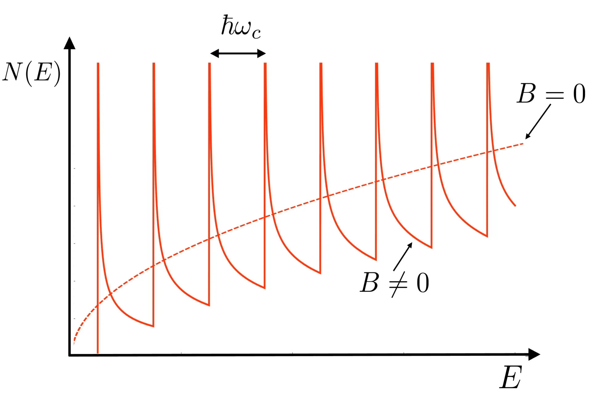
The energies correspond to a discrete set of one-dimensional systems, so that the density of states is determined by the structure of the one-dimensional dispersion (with square root singularities at the band edges) along the $z$ -direction:

\begin{aligned} N_{0} (E, n, s) & = \frac{N_{\deg}}{Ω} \sum_{k_{z}} δ (E - E_{n, k_{z}, s}) \\ = \frac{1}{2 π ℓ^{2}} \int \frac{d k_{z}}{2 π} δ (E - \frac{ℏ^{2} k_{z}^{2}}{2 m} - \underset{ϵ_{n, s}}{\underset{⏟}{[ℏ ω_{c} (n + \frac{1}{2}) - \frac{g μ_{B}}{ℏ} B s]}}) \\ = \frac{(2 m)^{3 / 2} ω_{c}}{8 π^{2} ℏ^{2}} \frac{1}{\sqrt{E - ϵ_{n, s}}} = \frac{3}{8} \frac{n}{ϵ_{F}} \frac{ℏ ω_{c}}{\sqrt{ϵ_{F}}} \frac{1}{\sqrt{E - ϵ_{n, s}}} \end{aligned}

The total density of states $N_{0} (E)$ for a given energy $E$ is obtained by summing over $n \in N_{0}$ and $s = \pm ℏ / 2$ . This should be compared to the density of states without the magnetic field,

\begin{array}{r} N_{0} (E, B = 0) = \frac{1}{Ω} \sum_{k, s} δ (E - \frac{ℏ^{2} | k |^{2}}{2 m}) = \frac{(2 m)^{3 / 2}}{2 π^{2} ℏ^{3}} \sqrt{E} . \end{array}

The density of states for finite applied field is shown for one spin-component:

Attachments/Script 38.webp|700

4.1.2 Oscillatory Behaviour of the Magnetisation

In the presence of a magnetic field, the smooth density of states of the three-dimensional metal is replaced by a discontinuous form dominated by square root singularities. The position of the singularities depends on the strength of the magnetic field. In order to understand the resulting effect on the magnetisation, we consider the free energy,

\begin{array}{r} F (N, T) = N μ - Ω (T, μ, B) = N μ - k_{B} T N_{\deg} \sum_{n, s} \int \frac{L d k_{z}}{2 π} \ln (1 + e^{- (E_{n, k_{z}, s} - μ) / k_{B} T}) \end{array}

with $Ω (T, μ, B)$ denoting the grand canonical potential and use the general thermodynamic relation $M = - \partial F (N, T) / \partial B$ . For the details of the somewhat tedious calculation, we refer to standard texts, for instance J. M. Ziman, Principles of the Theory of Solids, and merely present the result

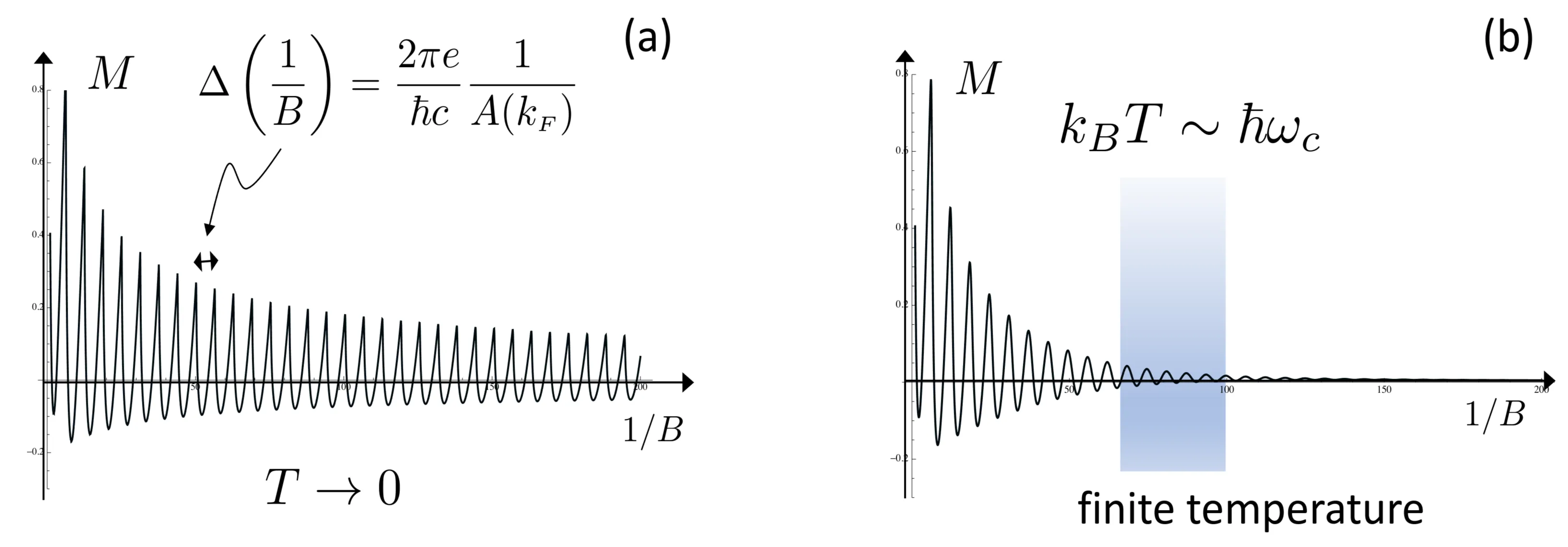
\begin{array}{r} M = χ_{P} B [1 + \frac{χ_{L}}{χ_{P}} + \frac{π k_{B} T}{μ_{B} B} \sqrt{\frac{ϵ_{F}}{μ_{B} B}} \sum_{ν = 1}^{\infty} \frac{1}{\sqrt{ν}} \frac{\sin (\frac{π}{4} - \frac{π ν ϵ_{F}}{μ_{B} B})}{\sinh (\frac{π^{2} ν k_{B} T}{μ_{B} B})}] . \end{array}

Here $χ_{P}$ is the Pauli-spin susceptibility originating from the Zeeman-term and the second term $χ_{L} = - χ_{P} / 3$ is the diamagnetic Landau susceptibility which is due to induced orbital currents (the Landau levels). For sufficiently low temperatures, $k_{B} T < μ_{B} B \sim ℏ ω_{c}$ , the magnetisation as a function of the applied field exhibits oscillatory behaviour:

Attachments/Script 39.webp|700

The dominant contribution comes from the summation with $ν = 1$ . The oscillations are a consequence of the singularities in the density of states that influence the magnetic moment upon successively passing through the Fermi energy as the magnetic field is varied. The period in $1 / B$ of the oscillations of the term $ν = 1$ is easily found to be

\begin{array}{r} \frac{π ϵ_{F}}{μ_{B}} Δ (\frac{1}{B}) = 2 π \end{array}

\begin{array}{r} Δ (\frac{1}{B}) = \frac{2 π e}{ℏ c A (k_{F})} \end{array}

where we used that $μ_{B} = ℏ e / (2 m c)$ and defined the cross sectional area $A (k_{F}) = π k_{F}^{2}$ of the Fermi sphere perpendicular to the magnetic field. Experimental data are often analyzed in terms of the de Haas-van Alphen frequency $F$ ,

\begin{array}{r} F = A (k_{F}) \frac{ℏ c}{2 π e} = \frac{A (k_{F}) Φ_{0}}{4 π^{2}} . \end{array}

4.1.3 Onsager Equation

The behaviour we have found above for a free electron gas, generalises to systems with arbitrary band structures. In these cases there are usually no exact solutions available. Instead of generalising the above treatment to such band systems, we discuss the behaviour of electrons within the semi-classical approximation, as introduced in Section 1.7, and consider the closed orbits of a wave packet subject to a magnetic field. The semi-classical equations of motion for the centre of mass of the wave packet simplify in the absence of an electric field to

\begin{aligned} \dot{r} & = v_{k} = \frac{\partial ϵ_{k}}{\partial ℏ k}, \\ ℏ \dot{k} & = - \frac{e}{c} v_{k} \times B . \end{aligned}

This defines a closed path in a plane perpendicular to the applied uniform magnetic field. The velocity $v_{k}$ stands perpendicular to lines of equal energy $ϵ_{k}$ . The electron follows in reciprocal space a path along such a line perpendicular to $B$ . The motion parallel to the magnetic field is independent with a constant $k_{∥}$ . Separating the motion parallel to $B$ the electrons move on a closed path in the perpendicular plane. Hence, we can apply the Bohr-Sommerfeld quantisation scheme yielding quantised closed paths $P_{n}$ (neglecting any uniform motion along the field direction),

\begin{array}{r} \oint_{P_{n}} p \cdot d r = h (n + γ) \end{array}

with $n$ being an integer and $γ$ a system specific shift, irrelevant for the final result and $h = 2 π ℏ$ . The canonical momentum within the semi-classical approach is expressed as $p = ℏ k - \frac{e}{c} A$ .
A common derivation using the relation $ℏ k_{p a t h} = - (e / c) (r_{p a t h} \times B)$ for the path momentum (relative to orbit centre) leads to:

\begin{aligned} \oint_{P_{n}} p \cdot d r & = - \frac{e}{c} \oint_{P_{n}} {A + (r \times B)} \cdot d r \\ = - \frac{e}{c} Φ_{n} + \frac{e}{c} B \cdot \oint_{P_{n}} r \times d r = - \frac{e}{c} Φ_{n} + \frac{e}{c} (2 Φ_{n}) = \frac{e}{c} Φ_{n} = h (n + γ), \end{aligned}

where $S_{n}$ is the area encircled by the path $P_{n}$ and $Φ_{n} = B_{⊥} S_{n}$ the magnetic flux threading it. With this we find

\begin{array}{r} Φ_{n} = (n + γ) Φ_{0} . \end{array}

Analogous to the real space also in reciprocal space the path of the electron encircles an area, $A_{n}$ . The relation between $S_{n}$ and $A_{n}$ can be derived from $ℏ d k = (e / c) (d r \times B)$ , leading to $S_{n} = (ℏ c / e B_{⊥})^{2} A_{n} = (Φ_{0} / (2 π B_{⊥}))^{2} A_{n}$ .
With the flux quantisation we obtain for a given magnetic field the area $A_{n}$ ,

\begin{array}{r} A_{n} = (n + γ) \frac{2 π e B_{⊥}}{ℏ c} = (n + γ) \frac{4 π^{2} B_{⊥}}{Φ_{0}} . \end{array}

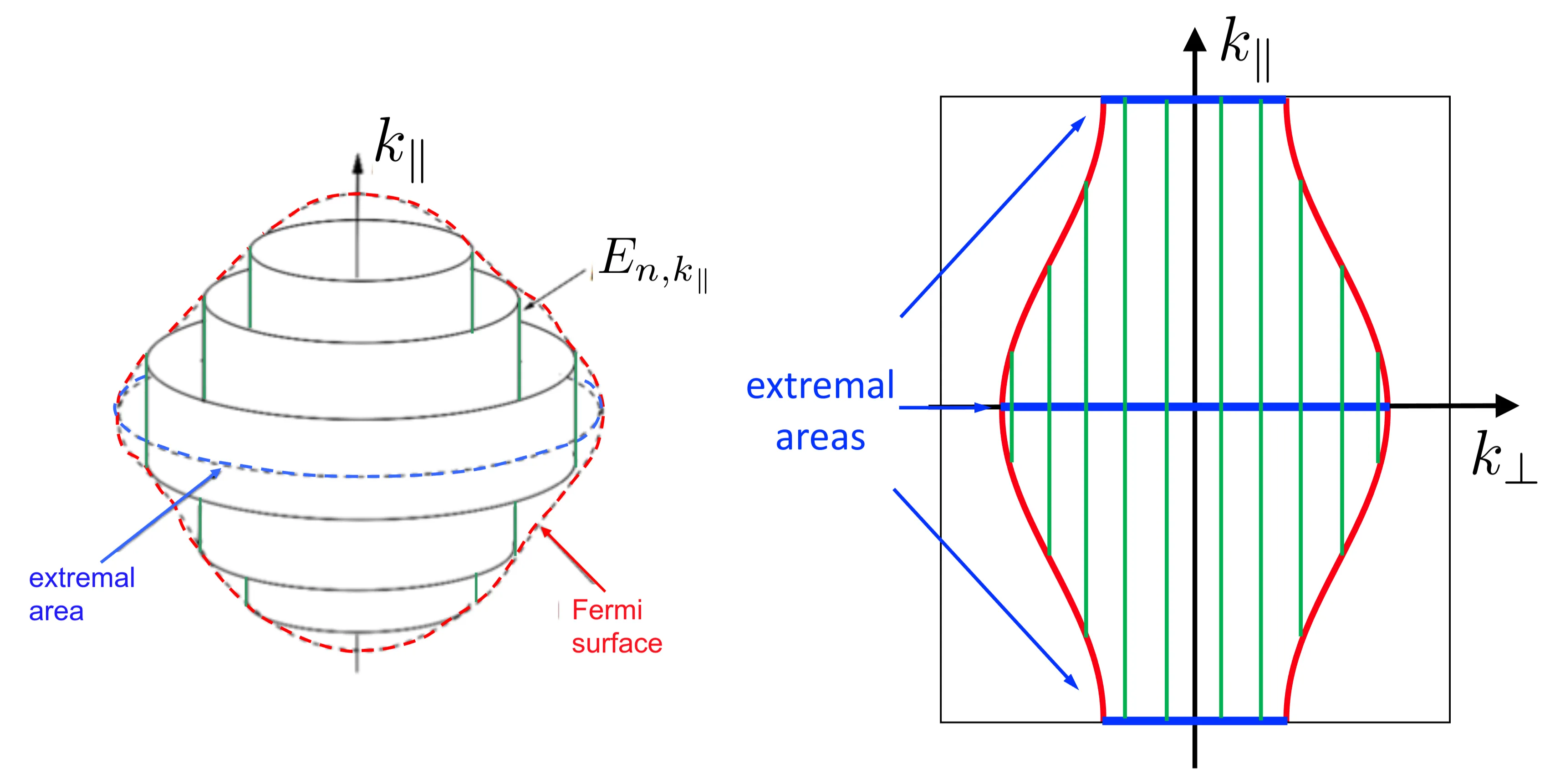
All the possible paths of given quantum number $n$ form cylinder-like surfaces parallel to $k_{∥}$ in reciprocal space, with energies $E_{n, k_{∥}}$ :

Attachments/Script 40.webp|700

Concentric tubes represent the quantised orbits in the reciprocal space corresponding to the areas $A_{n}$ embedded in the original Fermi surface which limits the height of the tubes, occupation along the $k_{∥}$ -direction $(k_{∥} ∥ B)$ . Left panel: 3-dimensional view of system with a simple Fermi surface. Right panel: cross section including $k_{z}$ . Extremal areas represent the band edges for the motion along $k_{∥}$ (bottom: maximal $A$ ; and top: minimal $A$ ).

The range of $k_{∥}$ for which this surface lies inside the filled Fermi sea is, thus, defined by $E_{n, k_{∥}} \leq ϵ_{F}$ . Different $n$ label different such concentric cylinders. The area between neighbouring paths depends linearly on $B_{⊥}$ ,

\begin{array}{r} A_{n + 1} - A_{n} = \frac{4 π^{2} B_{⊥}}{Φ_{0}} \end{array}

such that the densities of the cylinders decreases with increasing $B_{⊥}$ and the number of cylinders within the Fermi sea shrinks. Important are extremal cross sections of the Fermi sea perpendicular to $k_{∥}$ where a cylinder passes the Fermi surface. Such an extremal cross section corresponds to the top, bottom or saddle point of $ϵ_{k_{∥}}$ where the density of states has a singularities, analogous to the case of the band bottom of $ϵ_{k_{∥}} = ℏ^{2} k_{∥}^{2} / 2 m$ . If a cylinder hits such an extremal cross section a singularity of the density of states lies at the Fermi surface yielding a spike in the magnetisation.
For the extremal cross sectional area $A$ we ask what is the period between crossings of the cylinder. Thus, for different quantum numbers we find

\begin{array}{r} A = (n + γ) \frac{4 π^{2} B_{n}}{Φ_{0}} = (n^{'} + γ) \frac{4 π^{2}}{Φ_{0}} B_{n^{'}} . \end{array}

Thus changing the field $B$ from $B_{n}$ to $B_{n + 1}$ leads to two consecutive crossings. We observe that there is a regular oscillation as a function of $1 / B$ with the period,

\begin{array}{r} Δ (\frac{1}{B}) = \frac{1}{B_{n + 1}} - \frac{1}{B_{n}} = \frac{4 π^{2}}{A Φ_{0}} . \end{array}

We see in the left panel a Fermi surface with one extremal cross section. In the right panel there are three such cross sections. Such a vase-shaped Fermi surface may result from a band structure like,

\begin{array}{r} ϵ_{k} = \frac{ℏ^{2}}{2 m} (k_{x}^{2} + k_{y}^{2}) - 2 t \cos (k_{z} c) \end{array}

with $c$ the lattice constant along $z$ -axis. With $k_{∥}$ along the $z$ -axis. The cross sections are all circular parallel to $k_{x} - k_{y}$ -plane with a radius ${\tilde{k}}_{F} (k_{z})$ defined through

\begin{array}{r} {\tilde{k}}_{F} = \sqrt{\frac{2 m}{ℏ^{2}} (ϵ_{F} + 2 t \cos (k_{z} c))} . \end{array}

This yields a singularity in the density of states at the band top and bottom, such that

\begin{array}{r} N_{0} (E) = \frac{1}{4 π^{2} ℓ^{2} t} \sum_{n = 0}^{\infty} \frac{1}{\sqrt{1 - {(E - ϵ_{n, s})}^{2} / (2 t)^{2}}} . \end{array}

The oscillations in the magnetisation, thus, allow to measure the cross sectional area of the Fermi 'sphere'. By varying the orientation of the field the topology and shape of the Fermi surface can be mapped. As an alternative to the measurement of magnetisation oscillations one can also measure resistivity oscillations known under the name Schubnikov-de Haas effect. For both methods it is crucial that the Landau levels are sufficiently clearly recognisable. Apart from a low temperature this type of measurement requires sufficiently clean samples. In this context, "sufficiently clean" means that the average life-time $τ$ (average time between two scattering events) has to be much larger than the period of the cyclotron orbits, that is $ω_{c} τ ≫ 1$ . This condition follows from the uncertainty relation

\begin{array}{r} Δ ϵ \sim \frac{ℏ}{τ} ≪ ℏ ω_{c} . \end{array}

This means that one can improve the situation by going to high magnetic fields.

4.2 Quantum Hall Effect

Classical Hall Effect

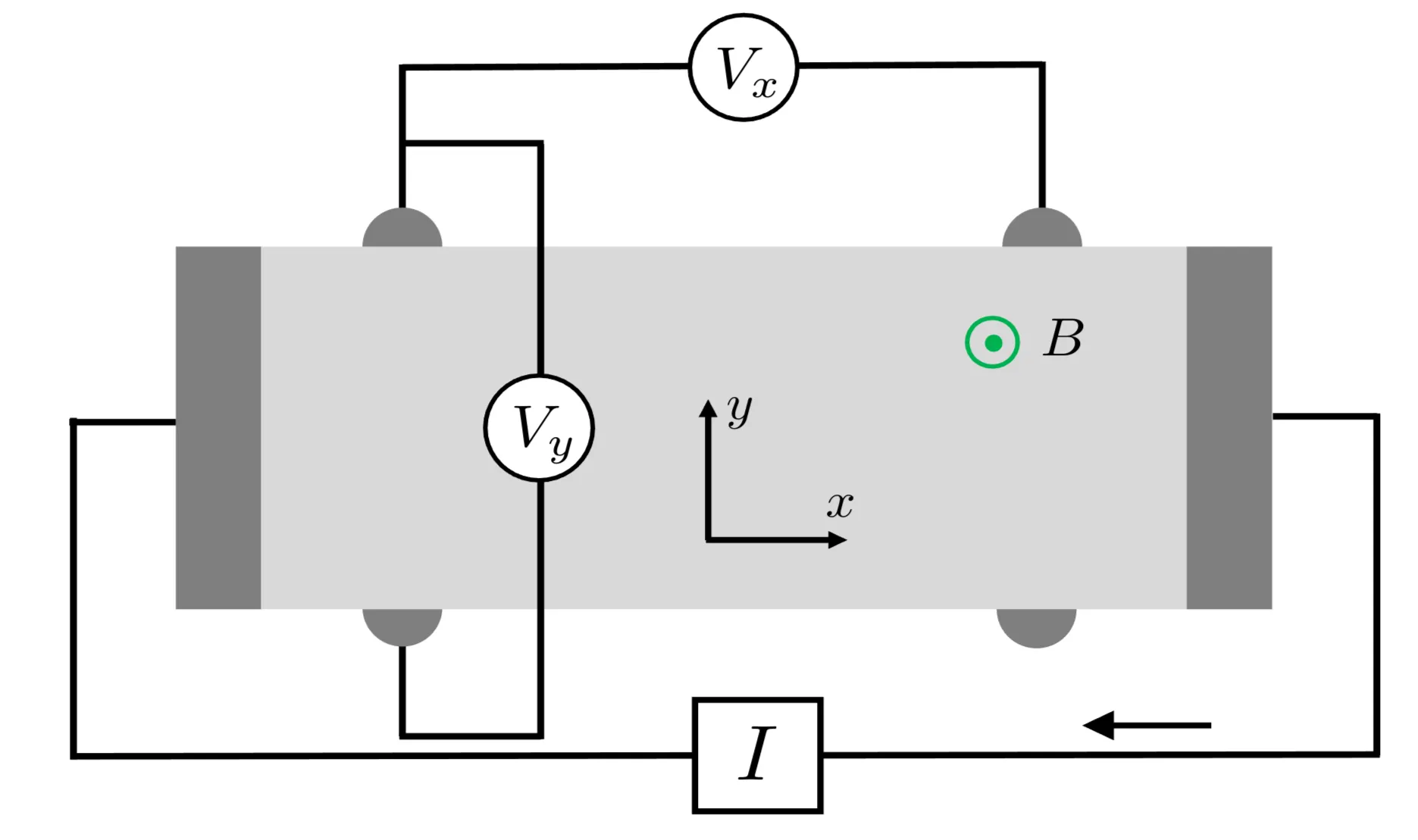
The Hall effect, discovered by Edwin Hall in 1879, originates from the Lorentz force exerted by a magnetic field on a moving charge. This force is perpendicular both to the velocity of the charged particle and to the magnetic field. In the presence of an electrical current, a Lorentz force produces a transverse voltage, whenever the applied magnetic field points in a direction non-collinear to the current in the conductor. This so-called Hall effect can be used to investigate some properties of the charge carriers. Before treating the quantum version, we briefly review the original Hall effect. To this end we consider the classical equation of motion of an electron, subject to an electric and a magnetic field

\begin{array}{r} m^{*} \frac{d v}{d t} = - e (E + \frac{v}{c} \times B) \end{array}

where $m^{*}$ is the effective electron mass and $e$ is the absolute value of the electron charge. For this classical system, the steady state equation reads

\begin{array}{r} E + \frac{v}{c} \times B = 0. \end{array}

Consider the Hall geometry here:

Attachments/Script 41.webp|700

Further, consider the fixed current $j = (j_{x}, 0, 0) = (- n_{0} e v_{x}, 0, 0)$ and magnetic field $B = (0, 0, B_{z})$ , this steady state condition simplifies to

\begin{array}{r} E_{y} - \frac{v_{x} B_{z}}{c} = 0. \end{array}

The solution $E_{y} = v_{x} B_{z} / c$ yields the Hall voltage that compensates the Lorentz force. The Hall conductivity $σ_{H}$ is defined as the ratio between the longitudinal current $j_{x}$ and the transverse electric field $E_{y} (j_{x} = σ_{x y} E_{y})$ , leading to

\begin{array}{r} σ_{H} = σ_{x y} = \frac{j_{x}}{E_{y}} = - \frac{n_{0} e c}{B_{z}} = ν \frac{e^{2}}{h} \end{array}

where $ν = - n_{0} h c / (B_{z} e)$ . We infer that the measurements of the Hall conductivity can be used to determine both the charge density $n_{0}$ and the sign of the charge carriers, that is whether the Fermi surface encloses the $Γ$ -point for electron-like, negative charges or a point on the boundary of the Brillouin zone for hole-like, positive charges.

Discovery of the Quantum Hall Effects

When measuring the Hall effect in a special two-dimensional electron system, Klaus von Klitzing and his collaborators made an astonishing discovery in 1980. The system was the inversion layer of GaAs-MOSFET device with a sufficiently high gate voltage (see MOSFET) which behaves like a two-dimensional electron gas with a high mobility $e τ / m^{*}$ due to the mean free path $l \sim 10 Å$ and low density $(n_{0} \sim 10^{11} {cm}^{- 2})$ . The two extended dimensions correspond to the interface of the MOSFET, whereas the electrons are confined in the third dimension like in a potential well. In high magnetic fields between $1 T - 30 T$ and at sufficiently low temperatures ( $T < 4 K$ ), von Klitzing and coworkers observed a quantisation of the Hall conductivity corresponding to exact integer multiples of $e^{2} / h$

\begin{array}{r} σ_{H} = ν_{n} \frac{e^{2}}{h} \end{array}

where $ν_{n} \in Z$ . By now, the integer quantisation is so widely verified, that the von Klitzing constant (resistance quantum named after the discoverer of the Quantum Hall effect) $R_{K} = h / e^{2} = 25812.807 Ω$ is used in resistance calibrations. In the field range where the transverse conductivity shows integer plateaus in $ν \sim 1 / B$ , the longitudinal conductivity $σ_{x x}$ vanishes and takes finite values only when $σ_{H}$ crossed over from one quantised value to the next:

Attachments/Script 42.webp|700

In 1982, Tsui, Störmer, and Gossard discovered an additional quantisation of $σ_{H}$ , corresponding to certain rational multiples of $e^{2} / h$ . Correspondingly, one now distinguishes between the integer quantum Hall effect (short: IQHE) and the fractional quantum Hall effect (short: FQHE). These discoveries marked the beginning of a whole new field in solid state physics that continues to produce interesting results.

4.2.1 Hall Effect of the Two-Dimensional Electron Gas

Here we first discuss the Hall effect in the quantum mechanical treatment. For this purpose we start with the Hamilton operator and neglect the electron spin. Working again in the Landau gauge, $A = (- B y, 0, 0)$ , and confining the electronic system to two dimensions, the Hamiltonian reduces to

\begin{array}{r} H = \frac{1}{2 m} [- ℏ^{2} \frac{\partial^{2}}{\partial y^{2}} + {(- i ℏ \frac{\partial}{\partial x} - \frac{e}{c} B y)}^{2}] . \end{array}

For the two-dimensional gas there is no motion in the $z$ -direction, so that the highly degenerate energy eigenvalues are given by the spectrum of a one-dimensional harmonic oscillator $E_{n} = ℏ ω_{c} (n + 1 / 2)$ , where again $ω_{c} = | e B | / m c$ . Here, we will concentrate on the lowest Landau level ( $n = 0$ ) with the wave function

\begin{array}{r} ϕ_{0, k_{x}} (x, y) = \frac{1}{\sqrt{L_{x} \sqrt{π} ℓ}} e^{- {(y - y_{0})}^{2} / 2 ℓ^{2}} e^{i k_{x} x} \end{array}

where the magnetic length $ℓ = \sqrt{ℏ c / | e B |}$ gives the extension of the wave function in the presence of the magnetic field, and $L_{x}$ is the length of the system in x-direction for normalization. In $y$ -direction, the wave function is localised around $y_{0} = k_{x} ℓ^{2}$ , whereas it takes the form of a plane wave in $x$ -direction. As discussed previously, the energy does not depend on $k_{x}$ .
We now introduce an electric field $E_{y}$ along the $y$ -direction. The Hamiltonian is then modified by an additional potential $U (r) = - e E_{y} y$ . This term can easily be absorbed into the harmonic potential and leads to a shift of the centre of the wave function,

\begin{array}{r} y_{0} (k_{x}) \to y_{0}^{'} (k_{x}) = k_{x} ℓ^{2} + \frac{e E_{y}}{m ω_{c}^{2}} . \end{array}

Moreover the degeneracy of the Landau level is lifted since the energy becomes $k_{x}$ -dependent and (after completing the square) takes the form

\begin{array}{r} E_{n = 0} (k_{x}) = \frac{ℏ ω_{c}}{2} - e E_{y} y_{0}^{'} (k_{x}) + \frac{m}{2} {(\frac{c E_{y}}{B})}^{2} . \end{array}

This energy corresponds to the wave function $ϕ_{0, k_{x}}$ (with $y_{0}$ replaced by $y_{0}^{'}$ ). The velocity of the electrons is then given by

\begin{array}{r} v_{x} (k_{x}) = \frac{1}{ℏ} \frac{d E_{n = 0} (k_{x})}{d k_{x}} = - \frac{e E_{y} ℓ^{2}}{ℏ} = - \frac{c E_{y}}{B}, \end{array}

and from this, we determine the current density,

\begin{aligned} j_{x} & = - e n_{0} v_{x} (k_{x}) = - e n_{0} (- \frac{c E_{y}}{B}) = \frac{e n_{0} c E_{y}}{B} . \end{aligned}

Using $n_{0} = ν / (2 π ℓ^{2})$ where $ν$ is the filling factor of the Landau level (number of electrons per degenerate state, $N_{0} / N_{\deg}$ ), we get

\begin{array}{r} j_{x} = \frac{e ν}{2 π ℓ^{2}} \frac{c E_{y}}{B} = \frac{e ν}{2 π (ℏ c / | e B |)} \frac{c E_{y}}{B} = ν \frac{e^{2} | B |}{2 π ℏ B} E_{y} = ν \frac{e^{2}}{h} E_{y} . \end{array}

So, $σ_{H} = ν \frac{e^{2}}{h}$ .
Note that $ν^{- 1} = B / (n_{0} Φ_{0})$ where $Φ_{0} = h c / e$ represents the flux quantum, that is $ν^{- 1} \sim B$ is the number of flux quanta $Φ_{0}$ per electron. The Hall conductivity is then consistent with the result derived previously based on the quasi-classical approximation, if we identify the classical $ν$ there with this filling factor. There is a linear relation between the Hall conductivity $σ_{H}$ and the index $ν \sim B^{- 1}$ .

4.2.2 Integer Quantum Hall Effect

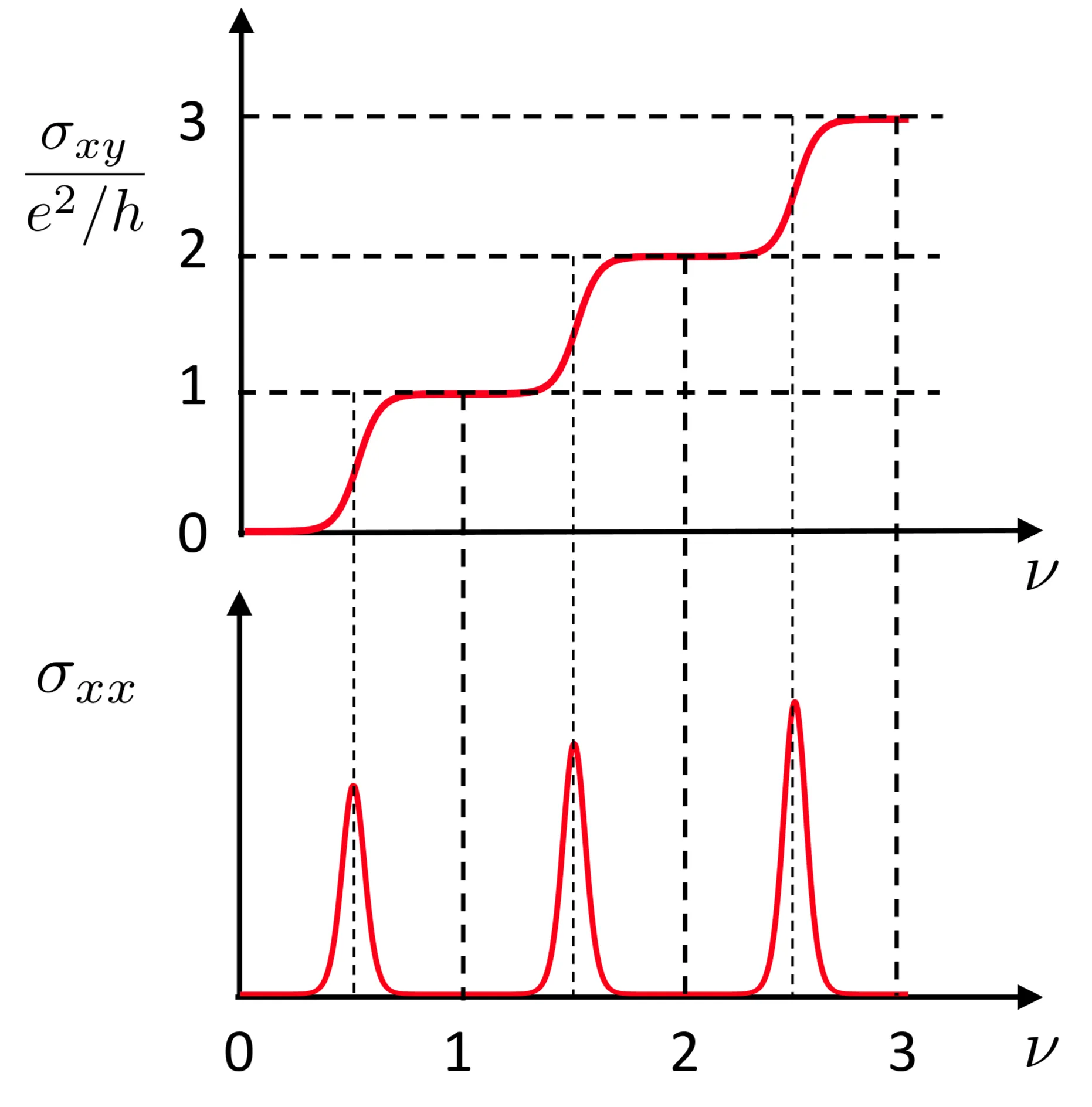
The plateaus observed by von Klitzing in the Hall conductivity $σ_{H}$ of the two-dimensional electron gas as a function of the magnetic field correspond to the values $σ_{H} = ν_{n} e^{2} / h$ , as if $ν = ν_{n} \in Z$ was restricted to be an integer. Meanwhile, the longitudinal conductivity of the electron gas vanishes when a plateau of $σ_{H}$ is realised

\begin{array}{r} σ_{x x} = \frac{j_{x}}{E_{x}} = 0 \end{array}

and only becomes finite at the transition points of $σ_{H}$ between two plateaus. This fact seems to be in contradiction with the results from the consideration above. The solution to this mysterious behaviour lies in the fact that disorder, which is always present in a real inversion layer, plays a crucial role and should not be neglected. In fact, due to the disorder, the electrons move in a randomly modulated potential landscape $U (x, y)$ . As we will find out, even small amounts of disorder lead to the localisation of electronic states in this two-dimensional system. To illustrate this new aspect we focus on the lowest Landau level in the symmetric gauge $A = \frac{B}{2} (- y, x, 0)$ (for $B > 0$ ). The Schrödinger equation in polar coordinates is given by

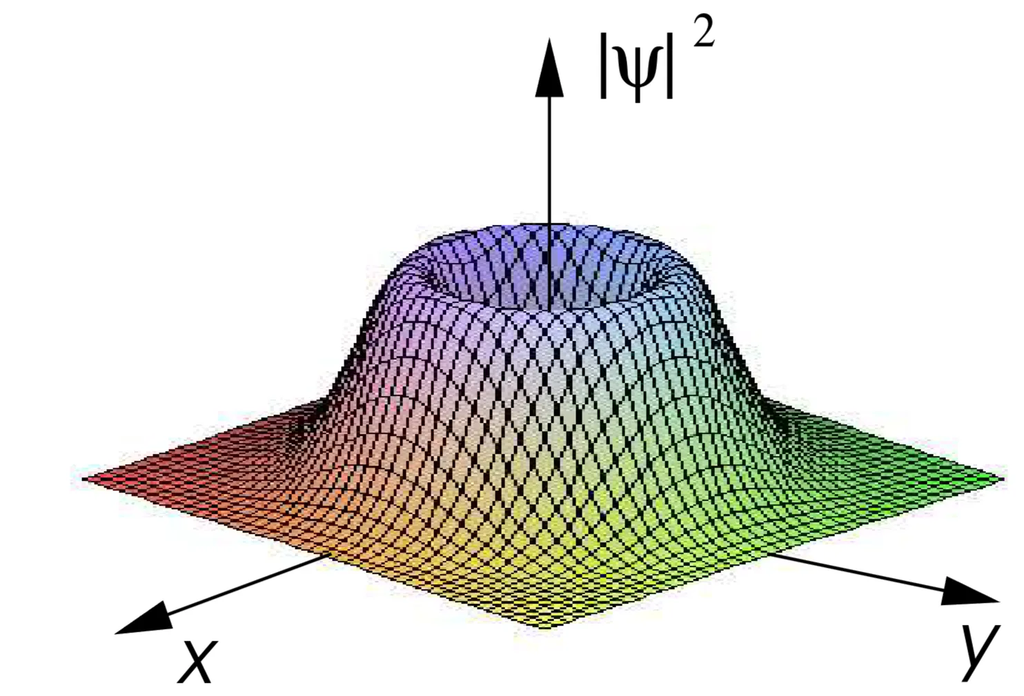
\begin{array}{r} \frac{ℏ^{2}}{2 m^{*}} [- \frac{1}{r} \frac{\partial}{\partial r} r \frac{\partial}{\partial r} - {(\frac{1}{r} \frac{\partial}{\partial φ} + i \frac{e B r}{2 ℏ c})}^{2}] ψ (r, φ) + U (x, y) ψ (r, φ) = E ψ (r, φ) . \end{array}

Without the external potential $U (x, y)$ we find the ground state solutions

\begin{array}{r} ψ_{n = 0, m} (r, φ) = \frac{1}{ℓ \sqrt{2 π 2^{m} m!}} {(\frac{r}{ℓ})}^{m} e^{- i m φ} e^{- r^{2} / 4 ℓ^{2}} \end{array}

where all values of $m \in N_{0}$ correspond to the same energy $E_{n = 0} = ℏ ω_{c} / 2$ . One easily verifies, that the wave functions $| ψ_{n = 0, m} (r, φ) |$ are peaked on circles of radius $r_{m} = \sqrt{2 m} ℓ$ :

Attachments/Script 43.webp|700

Note that the magnetic flux threading such a circle is given by

\begin{array}{r} π B r_{m}^{2} = π B 2 m ℓ^{2} = 2 π m B \frac{ℏ c}{e B} = m \frac{h c}{e} = m Φ_{0} \end{array}

which is an integer multiple of the flux quantum $Φ_{0} = h c / e$ .

Now we consider the effect of the disorder potential. The gauge can be adjusted to the potential landscape. If, for simplicity, we assume the potential to be rotationally invariant around the origin, the symmetric gauge is already optimal. For the potential

\begin{array}{r} U (x, y) = U (r) = \frac{C_{1}}{r^{2}} + C_{2} r^{2} + C_{3} \end{array}

the exact expression of all eigenstates of the Schrödinger equation in the lowest Landau level is obtained using the Ansatz

\begin{array}{r} {\tilde{ψ}}_{0, m} (r, φ) = \frac{1}{\sqrt{2 π (ℓ^{*})^{2} 2^{α} Γ (α + 1)}} {(\frac{r}{ℓ^{*}})}^{α} e^{- i m φ} e^{- r^{2} / 4 (ℓ^{*})^{2}} . \end{array}

After introducing the dimensionless parameters $C_{1}^{*} = 2 m^{*} C_{1} / ℏ^{2}$ and $C_{2}^{*} = 8 ℓ^{4} m^{*} C_{2} / ℏ^{2}$ , the quantities $α$ and $ℓ^{*}$ from the previous Ansatz can be expressed via

\begin{aligned} α^{2} & = m^{2} + C_{1}^{*}, \\ {(ℓ^{*})}^{- 2} & = (ℓ)^{- 2} \sqrt{1 + C_{2}^{*}} . \end{aligned}

Indeed, this Ansatz describes eigenstates of the disordered problem. The degeneracy of the ground state energy (the lowest Landau level) is now lifted,

\begin{array}{r} E_{0, m} = \frac{ℏ ω_{c}}{2} [\frac{ℓ^{2}}{(ℓ^{*})^{2}} (α + 1) - m] + C_{3} . \end{array}

The wave functions are concentrated around the radii $r_{m} = \sqrt{2 α} ℓ^{*}$ . For weak potentials $C_{1}^{*}, C_{2}^{*} ≪ 1$ and $m ≫ 1$ the energy is approximatively given by

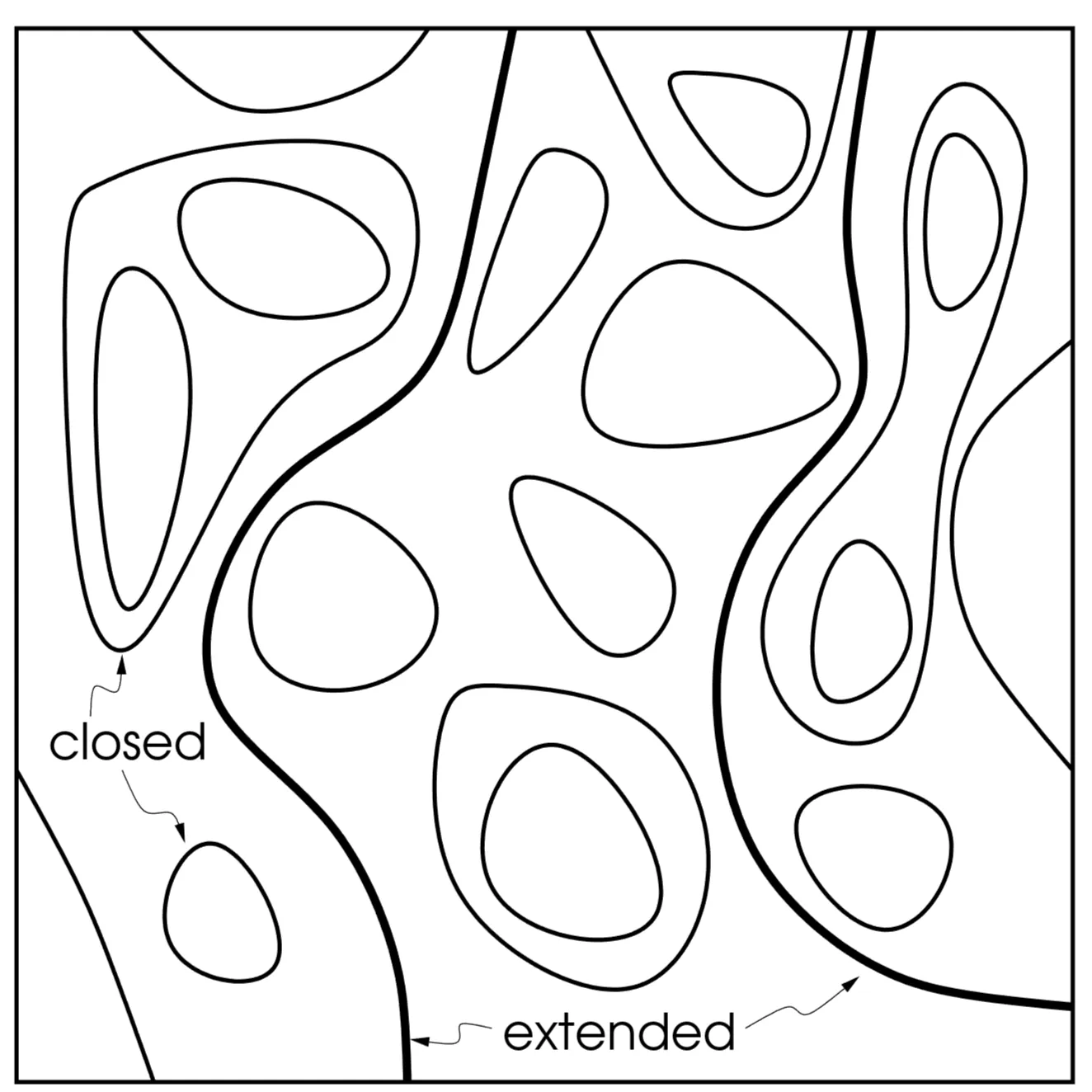
\begin{array}{r} E_{0, m} \approx \frac{ℏ ω_{c}}{2} + \frac{C_{1}}{r_{m}^{2}} + C_{2} r_{m}^{2} + C_{3} + \dots \end{array}

that is the wave function adjusts itself to the potential landscape. It turns out that the same is true for arbitrarily structured weak potential landscapes. The wave function describes electrons on quasi-classical trajectories that trace the equipotential lines of the underlying disorder potential. Consequently the states described here are localised in the sense that they are attached to the structure of the potential. The application of an electric field cannot set the electrons in the concentric rings in motion. Therefore, the electrons are localised and do not contribute to electric transport.

Picture of the potential landscape

When the magnetic field is varied the filling $ν = n_{0} 2 π ℓ^{2}$ of the Landau level is adjusted accordingly. While all states of a given level are degenerate in the transitionally invariant case, now, these states are spread over a certain energy range due to the disorder. In the quasi-classical approximation, these states correspond to equipotential trajectories that are either filled or empty depending on the strength of the magnetic field, that is they are either below or above the chemical potential. These considerations lead to an intuitive picture on localised (closed trajectories) and extended (percolating trajectories) states. We may consider the potential landscape like a real landscape where the trajectories are contour lines. Assume that we fill now water into such a landscape. The trajectories of the particles is restricted to the shore line. For small filling, we find lakes whose shores are closed and correspond to contour lines. They correspond to closed electron trajectories and represent localised electronic states. At very high water level, only the large mountains of the potential landscape would reach out of the water, forming islands in the sea. The coastlines again represent closed trajectories corresponding to localised electronic states. At some intermediate filling, a boundary between the lake and the island topology, there is a water level at which the coast lines become arbitrarily long and percolate through the whole landscape. Only these contour lines correspond to extended (non-localised) electron states. From this picture we conclude that when a Landau level of a system subject to a random potential is gradually filled, first all occupied state are localised (low filling). At some special intermediate filling level, the extended states are filled and contribute to the current transport. At higher chemical potential (filling) the states would be localised again. In the following argument, going back to Robert B. Laughlin, the presence of filled extended states plays an important role.

Attachments/Script 44.webp|700

Laughlin's gauge argument

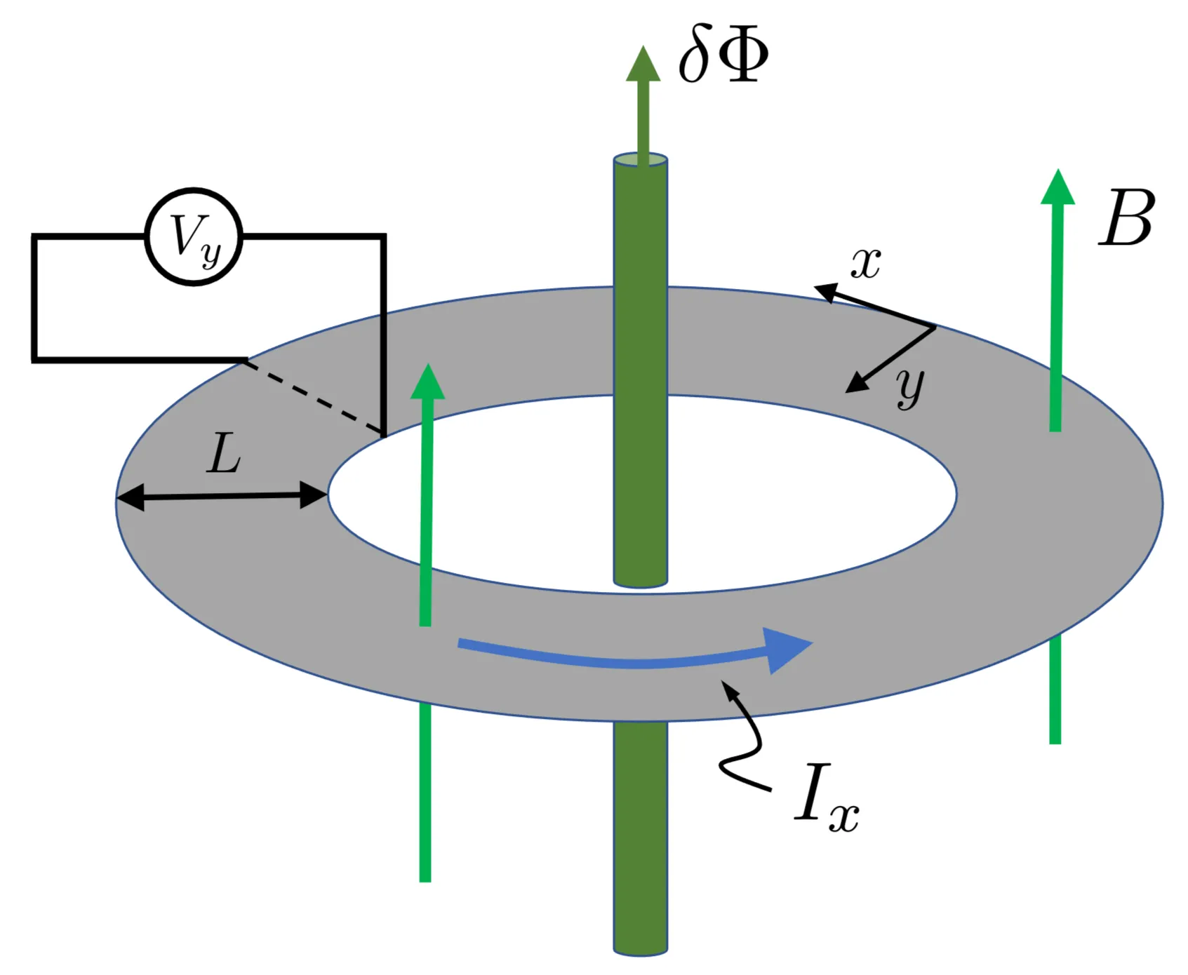
We consider a long rectangular Hall element that is deformed into a so-called Corbino disc, that is a circular disc with a hole in the middle as shown here:

Attachments/Script 45.webp|700

The Hall element is threaded by a constant and uniform magnetic field $B$ along the $z$ -axis. In addition we can introduce an arbitrary flux $Φ$ through the hole without influencing the uniform field in the disc. This flux is irrelevant for all localised electron trajectories since only extended (percolating) trajectories wind around the hole of the disc and by doing so receive an Aharonov-Bohm phase. When the flux is increased adiabatically by $δ Φ$ , the vector potential is changed according to

\begin{array}{r} A \to A + δ A = A + \nabla χ \end{array}

which in our case means

\begin{array}{r} (δ A)_{φ} = \frac{δ Φ}{2 π r} . \end{array}

At the same time, the wave function acquires a phase factor

\begin{array}{r} ψ \to ψ e^{- i e χ / (ℏ c)} = ψ e^{- i (δ Φ / Φ_{0}) φ} . \end{array}

If the disc was translationally invariant, meaning that disorder is neglected and only extended states exist, we could use the wave functions $ψ_{0, m}$ previously discussed, so that $B π r_{m}^{2} = m Φ_{0} + δ Φ$ . The single-valuedness of the wave function implies that $m$ has to be adjusted, $m \to m - δ Φ / Φ_{0}$ . This guarantees, that increasing $Φ$ by one flux quantum leads to a decrease of $m$ by 1. Hence, gauge invariance implies that the wave functions are shifted in their radius. This argument is also applicable to higher Landau levels.
Since this argument is topological in nature, it will not break down for independent electrons when disorder is introduced. The transfer of one electron between neighbouring extended states due to the change of $Φ$ by $Φ_{0}$ leads to a net shift of one electron from the outer to the inner boundary. If an electric field $E_{y}$ is applied in the radial direction (here denoted by $y$ -direction), the transfer of this electron (charge $- e$ ) results in the energy change

\begin{array}{r} Δ E_{V} = (- e) E_{y} L \end{array}

where $L$ is the distance between the inner and the outer boundary of the Corbino disc. A further change in the electromagnetic energy

\begin{array}{r} Δ E_{I} = \frac{I_{x} δ Φ}{c} \end{array}

is caused by the constant current $I_{x}$ (here the angular component is denoted by $x$ ) in the disc when the magnetic flux is increased by $δ Φ$ . Following the Aharonov-Bohm argument that the energy of the system is invariant under a flux change by integer multiples of $Φ_{0}$ , the two energies should compensate each other. Thus, setting $δ Φ = Φ_{0}$ and demanding that $Δ E_{V} + Δ E_{I} = 0$ leads to $- e E_{y} L + I_{x} Φ_{0} / c = 0$ , so $I_{x} = e c E_{y} L / Φ_{0} = e c E_{y} L / (h c / e) = (e^{2} / h) E_{y} L$ . The Hall conductivity is then

\begin{array}{r} σ_{H} = \frac{j_{x}}{E_{y}} = \frac{I_{x} / L}{E_{y}} = \frac{e^{2}}{h} . \end{array}

We conclude from this argument, that each filled Landau level containing percolating states will contribute $e^{2} / h$ to the total Hall conductivity.
Alternative view point: We assume that the flux $δ Φ$ changes linearly in time, $δ Φ (t) = t Φ_{0} / T_{0}$ introducing in the time $T_{0}$ one flux quantum $(T_{0} ω_{c} ≫ 1)$ . Looking at a concentric circle of radius $R$ on the Corbino disc, we can define an azimutal electric field due to the Faraday effect,

\begin{array}{r} 2 π R E_{ϕ} = - \frac{1}{c} \frac{\partial δ Φ}{\partial t} = - \frac{Φ_{0}}{c T_{0}} . \end{array}

At the same time one electron (per filled Landau level) is moved inwards, such that we define the mean current density $j_{r}$ as

\begin{array}{r} I_{r} = 2 π R j_{r} = - \frac{e}{T_{0}} . \end{array}

This allows us to define the Hall conductance,

\begin{array}{r} σ_{x y} = \frac{j_{y}}{E_{x}} = \frac{j_{r}}{E_{ϕ}} = \frac{- e / (T_{0} 2 π R)}{- Φ_{0} / (c T_{0} 2 π R)} = \frac{c e}{Φ_{0}} = \frac{e^{2}}{h} \end{array}

for each filled Landau level.
Hence, for $ν_{n} \in N$ filled levels the Hall conductivity is given by $σ_{H} = ν_{n} e^{2} / h$ . Note the importance of the topological nature of the Hall conductivity ensuring the universal character of the quantisation.

Localised and extended states

The density of states of the two-dimensional electron gas (2DEG) in absence of an external magnetic field is given by

\begin{array}{r} N_{2 DEG} (E) = 2 \sum_{k_{x}, k_{y}} δ (E - \frac{ℏ^{2} (k_{x}^{2} + k_{y}^{2})}{2 m}) = \frac{L_{x} L_{y} m}{π ℏ^{2}} \end{array}

with twice degenerate energy states for the spins, whereas for the Landau levels in a clean sample, we have

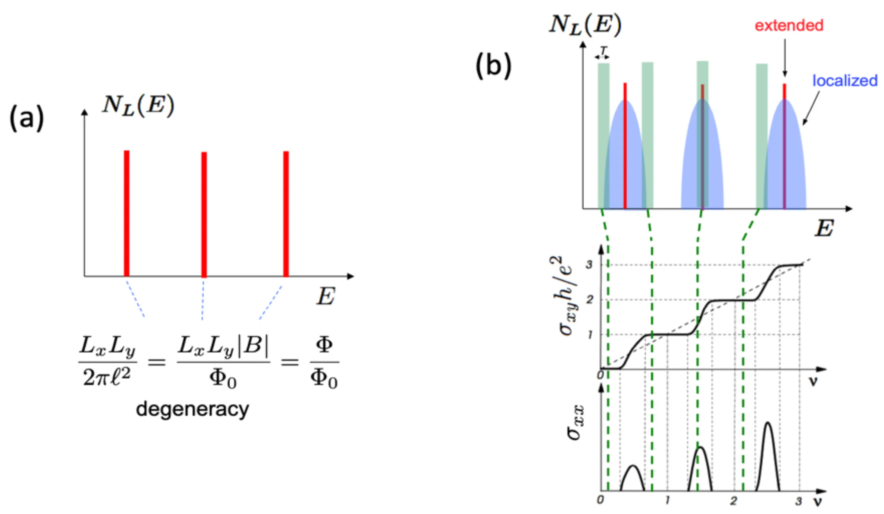
\begin{array}{r} N_{L} (E) = \frac{L_{x} L_{y}}{2 π ℓ^{2}} \sum_{n, s} δ (E - E_{n, s}) . \end{array}

Here the prefactor is given by the large degeneracy of each Landau level.

Attachments/Script 46.webp|700

The figure shows in (a) the density of states for the two-dimensional electron gas in a magnetic field. The Landau levels are infinitely sharp and have all identical degeneracy. In (b), with disorder the previously sharp Landau levels broaden in energy. Many states form in the random potential landscape closed semiclassical orbits which are, thus, localised. On the other hand, in the centre there are a few percolating extended semiclassical orbitals. Note that the number of states in each broadened Landau level is still the same as the original degeneracy. With varying magnetic field the chemical potential (here green bar with finite width $k_{B} T$ indicating broadened Fermi-Dirac distribution) moves, such that states below are filled and states above are empty. If the green bar is in the localised region all $ν_{n}$ lower Landau levels are completely filled and contribute $ν_{n} e^{2} / h$ to the Hall conductance $σ_{x y}$ which is in a plateau. All extended states are either completely filled or empty such that the system is insulating, that is $σ_{x x} = 0$ . If the chemical potential lies at the extended states of a Landau level these are partially filled and act metallic. Because the Landau level is only partially filled, the $σ_{x y}$ lies between two plateaus. Note that the width of the step between two plateaus of $σ_{x y}$ depends on temperature and shrinks with lowering temperature.

According to our previous discussion, the main effect of a potential is to lift the degeneracy of the states comprising a Landau level. This remains true for random potential landscapes. Most of the states are then localised and do not contribute to electric transport. Only the few extended states contribute to the transport if they are filled. For partially filled extended states the Hall conductivity $σ_{H}$ is not an integer multiple of $e^{2} / h$ , since not all percolating states - necessary for transferring one electron from one edge to the other, when the flux is changed by $Φ_{0}$ (in Laughlin's argument) - are occupied. Thus, the charge transferred does not amount to a complete $- e$ . The appearance of partially filled extended states marks the transition from one plateau to the next and is accompanied by a finite longitudinal conductivity $σ_{x x}$ . When all extended states of a Landau level are occupied, the contribution to the longitudinal transport stops, that is, in the range of a plateau $σ_{x x}$ vanishes. Because of thermal occupation, the plateaus quickly shrink when the temperature of the system is increased. This is the reason why the Quantum Hall Effect is only observable for sufficiently low temperatures ( $T < 4 K$ ).

Edge states and Büttiker's argument

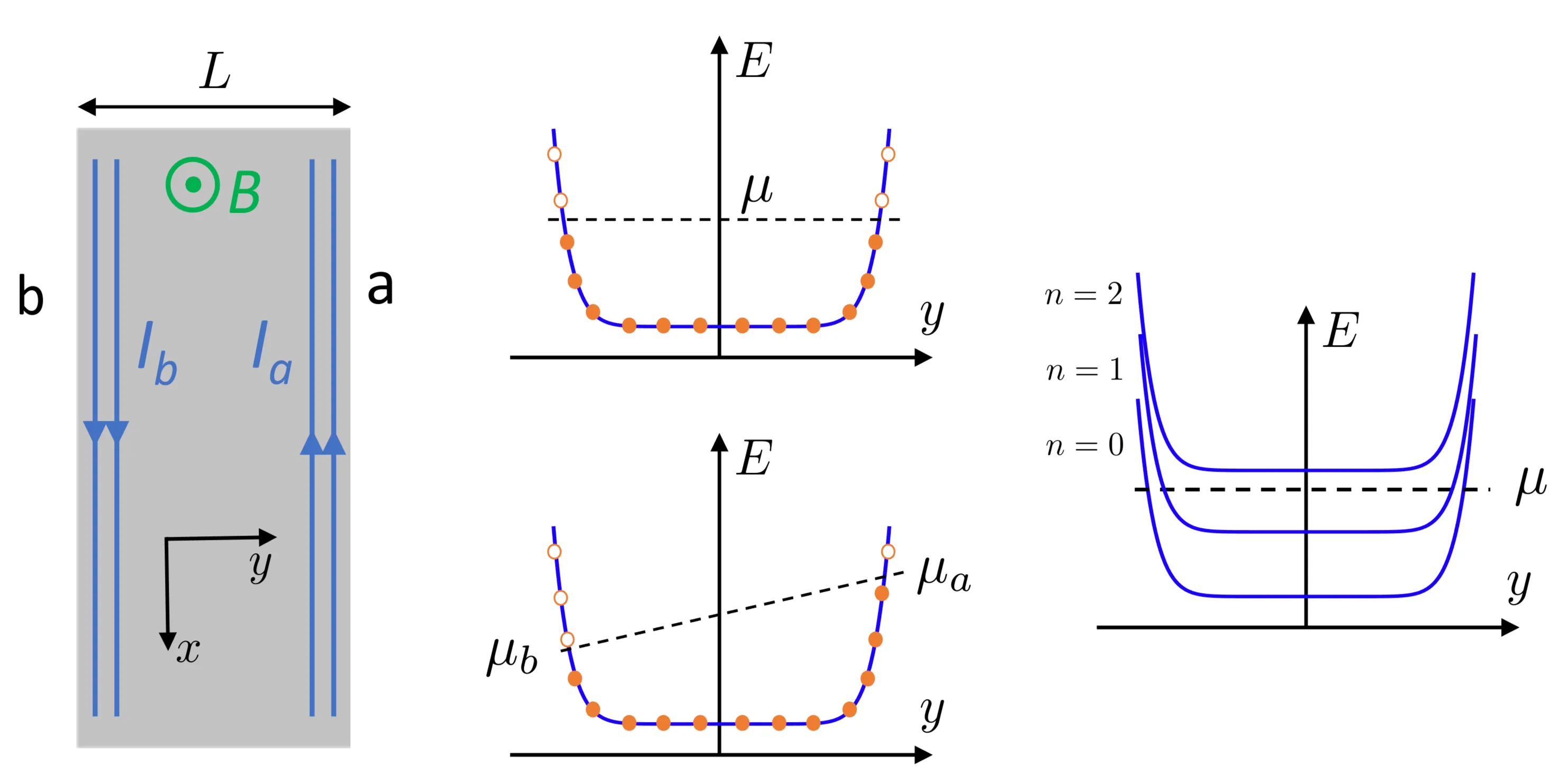
A confining potential prevents the electrons from leaving the metal. This potential at the edges of the sample has also to be considered in the potential landscape. Interestingly, equi-potential trajectories of states close to the edge are always extended and percolate along the edge. The corresponding wave functions have already been discussed. We find that the energy is not symmetric in $k_{y}$ , the wave vector along the edge, that is $E (k_{y}) \neq E (- k_{y})$ . This implies that the states are chiral and can move in one direction only for a given energy. The edge states on the opposing edges move in opposite directions, a fact that can be readily verified by inspection of the energy expression for states in crossed fields based on the figure below.
The total current flowing along an edge for a given Landau level is

\begin{array}{r} I = - \sum_{k_{x}}^{occ.} \frac{e}{L_{x}} v_{x} \end{array}

where we sum over all occupied states and each state labelled by $k_{x}$ (determining the corresponding centre $y_{0}$ ) extends over the whole length $L_{x}$ of the Hall element. Thus, the density is given by $1 / L_{x}$ . The wave vector is quantised according to the periodic boundary conditions; $k_{x} = 2 π n_{x} / L_{x}$ with $n_{x} \in Z$ . The velocity $v_{x}$ is given by the derivative of the energy with respect to $k_{x}$ . Thus, we have

\begin{aligned} I & = - \frac{e}{2 π ℏ} \int_{occupied} d k_{x} \frac{d E_{n} (k_{x})}{d k_{x}} \\ = - \frac{e}{h} \int_{occupied} d y_{0} \frac{d E_{n}}{d y_{0}} = - \frac{e}{h} (μ - E_{n}^{(0)}) \end{aligned}

where $y_{0} = k_{x} ℓ^{2}$ is the transversal position of the wave function and $μ$ is the chemical potential. Sufficiently far away from the boundary $E_{n}$ is independent of $y_{0}$ and approaches the value $E_{n}^{(0)} = ℏ ω_{c} (1 / 2 + n)$ of a translationally invariant electron gas.
Now we consider the geometry of the Hall bar with two edges:

Attachments/Script 47.webp|700

The potential difference between the two opposing edges leads to a net current along the edge direction of the Hall bar,

\begin{array}{r} I_{x} = - \frac{e}{h} (μ_{a} - μ_{b}) . \end{array}

If $μ_{a} - μ_{b} = - e V_{H} = - e (- E_{y} L_{y}) = e E_{y} L_{y}$ , then $I_{x} = - \frac{e}{h} (e E_{y} L_{y}) = - \frac{e^{2}}{h} E_{y} L_{y}$ .
And with that

\begin{array}{r} σ_{H} = \frac{I_{x}}{E_{y} L_{y}} = \frac{j_{x}}{E_{y}} = - \frac{e^{2}}{h}, \end{array}

where for $μ_{a} = μ_{b}$ we have $I_{a} = - I_{b}$ . Note that $I_{x} = I_{a} + I_{b}$ is only valid when no currents are present in the bulk of the system. The latter condition is ensured by the localisation of the states at the chemical potential. This argument by Büttiker leads to the same quantisation as derived before, namely every Landau level contributes one edge state and thus $σ_{H} = - ν_{n} e^{2} / h$ where $ν_{n}$ is the number of occupied Landau levels. Note that this argument is independent of the precise shape of the confining edge potential.
Within this argument we are able to understand why the longitudinal conductivity has to vanish at the Hall plateaus. For that we express Ohm's law. However it is simpler to discuss the resistivity. Like the conductivity $\hat{σ}$ the resistivity $\hat{ρ}$ is a tensor:

\begin{aligned} j & = \hat{σ} E \\ E & = \hat{ρ} j \end{aligned}

where the conductivity $\hat{σ}$ and the resistivity $\hat{ρ}$ are both $2 \times 2$ tensors with $σ_{x x} = σ_{y y} (ρ_{x x} = ρ_{y y})$ and $σ_{x y} = - σ_{y x} (ρ_{x y} = - ρ_{y x})$ . Therefore, we find

\begin{aligned} σ_{x x} & = \frac{ρ_{x x}}{ρ_{x x}^{2} + ρ_{x y}^{2}}, \\ σ_{x y} & = \frac{- ρ_{x y}}{ρ_{x x}^{2} + ρ_{x y}^{2}} . \end{aligned}

In the following argument, we explain why the longitudinal resistivity $ρ_{x x}$ in two dimensions has to vanish in the presence of a finite Hall resistivity $ρ_{x y}$ . Since the edge state electrons with a given energy can only move in one direction, there is no backward scattering by obstacles as long as the edges are far apart from each other. No scattering between the two edges implies $ρ_{x x} = 0$ and hence $σ_{x x} = 0$ . A finite resistivity can only occur when extended states are present in the bulk, such that the edge states on opposite edges are no longer spatially separated from each other.

4.2.3 Fractional Quantum Hall Effect

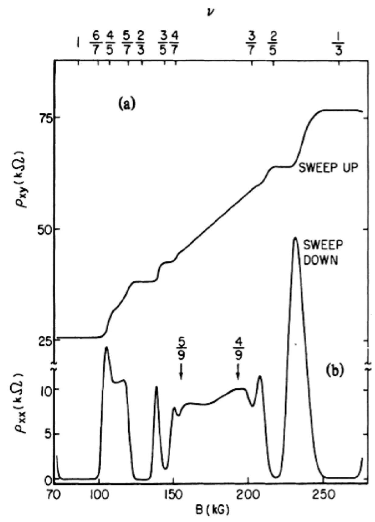
Only two years after the discovery of the Integer Quantum Hall Effect, Störmer, Tsui and Gossard observed further series of plateaus of the Hall resistivity in a 2DEG with very high quality MOSFET inversion layers at low temperatures:

Attachments/Script 48.webp|700

The most pronounced of these plateaus is observed at a filling of $ν = 1 / 3 (σ_{x y} = ν e^{2} / h)$ . Later, an entire hierarchy of plateaus at fractional values $ν = ν_{p, m} = p / m$ with $p, m \in N$ has been discovered,

\begin{array}{r} ν_{p, m} \in {\frac{1}{3}, \frac{2}{3}, \frac{2}{5}, \frac{3}{5}, \frac{3}{7}, \dots} . \end{array}

The emergence of these new plateaus is a clear evidence of the so-called Fractional Quantum Hall Effect (FQHE). It was again Laughlin who found the key concept to explain the FQHE. Unlike the IQHE, this new quantisation feature can not be understood from a single-electron picture, but is based on the Coulomb repulsion among the electrons and the accompanying correlation effects. Laughlin specially investigated the case $ν_{p, m} = 1 / 3$ and made Laughlin's Ansatz

\begin{array}{r} Ψ_{1 / m} (z_{1}, \dots, z_{N}) \sim \prod_{i < j} {(z_{i} - z_{j})}^{m} \exp (- \sum_{i} \frac{{| z_{i} |}^{2}}{4 ℓ^{2}}) \end{array}

for the $N$ -body wave function, where $z = x - i y$ is a complex number representing the coordinates of the two-dimensional system. Limiting ourselves to the consideration of the lowest Landau level, this state gives a stable plateau with $σ_{H} = (1 / 3) e^{2} / h$ , when $m = 3$ .
A heuristic interpretation of the Laughlin state was proposed by J. K. Jain and it is based on the concept of so-called composite Fermions. In fact, Laughlin's state can be written as

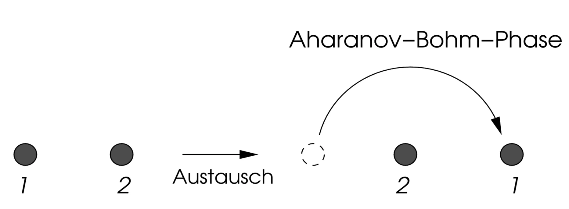
\begin{array}{r} Ψ_{1 / m} = \prod_{i < j} {(z_{i} - z_{j})}^{m - 1} Ψ_{S} \end{array}

where $Ψ_{S}$ is the Slater determinant describing the completely filled lowest Landau level. We see that the prefactor of $Ψ_{S}$ in this expression acts as a so-called Jastrow factor that introduces correlation effects into the wave function, since only the correlations due to the Pauli exclusion principle are contained in $Ψ_{S}$ . The Jastrow factor treats the Coulomb repulsion among the electrons and consequently leads to an additional suppression of the wave function whenever two electrons approach each other. In the form introduced above, it produces an phase factor for the electrons encircling each other. In particular, exchanging two electrons leads to a phase

\begin{array}{r} \exp (i (m - 1) π) = \exp (i \frac{e}{ℏ c} \frac{m - 1}{2} Φ_{0}), \end{array}

since $Φ_{0} = 2 π ℏ c / e$ . This phase has to be unity since the Slater state $Ψ_{S}$ is odd under exchange of two electrons.

Attachments/Script 49.webp|700

Therefore $m$ is restricted to odd integer values. This guarantees that the total wave function $Ψ_{1 / m}$ still changes sign when two electrons are exchanged.
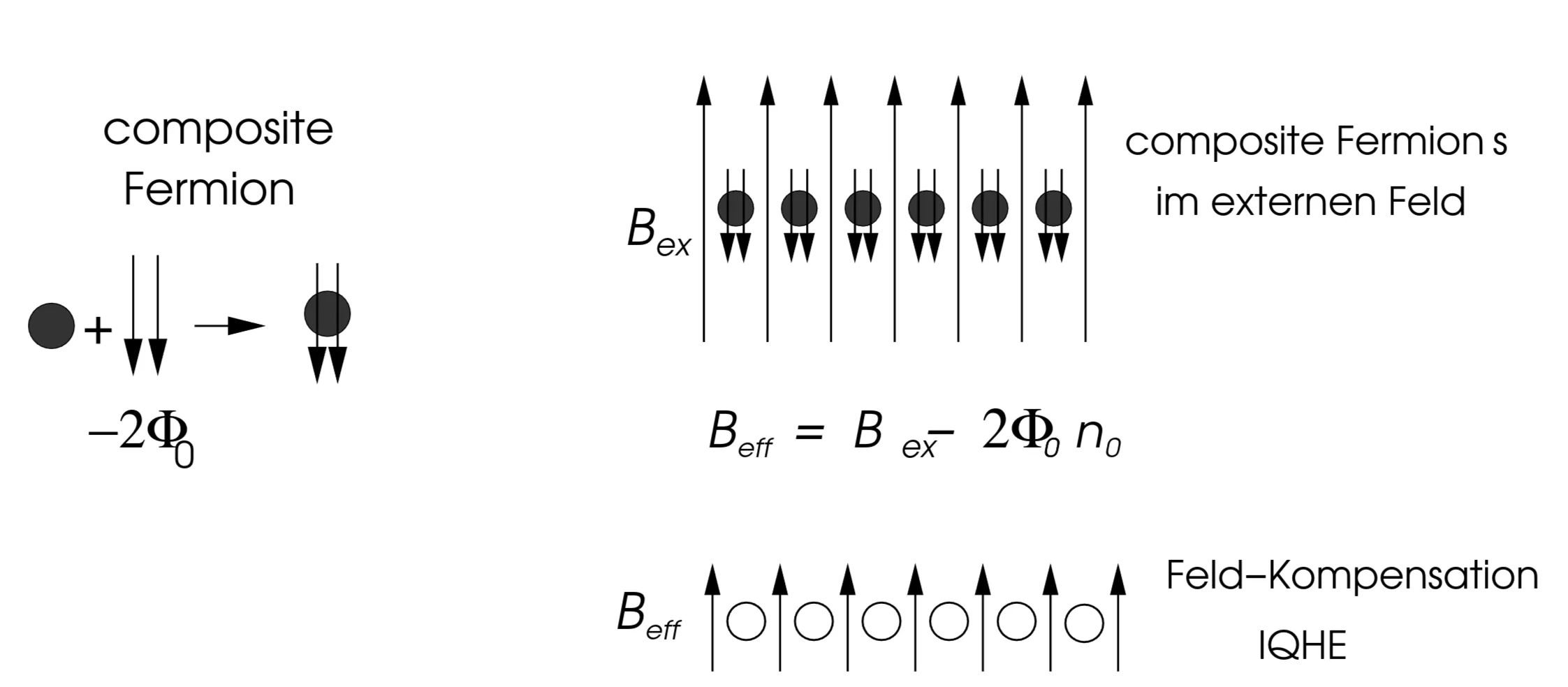
According to the relation between filling factor and flux quanta (previously $ν^{- 1} = B / (n_{0} Φ_{0})$ ), the case $ν_{p, m} = 1 / 3$ implies that there are three flux quanta $Φ_{0}$ per electron. In order to understand the FQHE, one constructs so-called composite Fermions which do not interact with each other. Here, a composite Fermion consists of an electron that has two (in fact $m - 1$ ) negative flux quanta attached to it. These objects may be considered as independent Fermions since the attached flux quanta compensate the Jastrow factor through factors of the type ${(z_{i} - z_{j})}^{- (m - 1)}$ . The exchange of two such composite Fermions in two dimensions leads to an Aharonov-Bohm phase that is just opposed to the phase derived earlier. Due to the presence of the flux $- 2 Φ_{0}$ per electron, the composite Fermions are subject to an effective field composed of the external field and the attached flux quanta:

\begin{aligned} B_{eff} & = B - 2 n_{C F} Φ_{0} \\ = \frac{1}{ν} n_{e} Φ_{0} - 2 n_{e} Φ_{0} = n_{e} Φ_{0} (\frac{1}{ν} - 2) \end{aligned}

where $n_{C F} = n_{e}$ is the density of composite fermions (equal to electron density). For $ν = 1 / 3$ , $B_{e f f} = n_{e} Φ_{0} (3 - 2) = n_{e} Φ_{0}$ .
For an external field $B = (1 / ν) n_{0} Φ_{0}$ , for $ν = 1 / 3$ , this is $B = 3 n_{0} Φ_{0}$ . The composite Fermions feel an effective field $B_{eff} = n_{0} Φ_{0}$ :

Attachments/Script 50.webp|700

Thus, these Fermions form an Integer Quantum Hall state with effective filling $ν_{e f f} = 1$ (for $B = 3 n_{0} Φ_{0}$ ), as discussed previously. This way of interpretation is applicable to other Fractional Quantum Hall states, too, since for $n$ filled Landau levels with composite Fermions consisting of an electron with an attached flux of $- 2 k Φ_{0}$ (where $2 k = m - 1$ ), the effective field implies a relation for the filling factors.
From this we infer, that

\begin{array}{r} \frac{1}{ν_{p, m}} = 2 k \pm \frac{1}{n} \end{array}

or equivalently (for the principal series with $\pm 1 / n$ )

\begin{array}{r} ν_{p, m} = \frac{p}{m} = \frac{n}{2 k n \pm 1} . \end{array}

Despite the apparent simplicity of the treatment in terms of independent composite Fermions, one should keep in mind that one is dealing with a strongly correlated electron system. The structure of the composite Fermions is a manifestation of the fact that the Fermions are not independent electrons. No composite Fermions can exist in the vacuum, they can only arise within a certain many-body state. The Fractional Quantum Hall state also exhibits unconventional excitations with fractional charges. For example, in the case $ν_{p, m} = 1 / 3$ , there are excitations with effective charge $e^{*} = e / 3$ . These are so-called 'topological' excitations, that can only exist in correlated systems. The Fractional Quantum Hall system is a very peculiar 'ordered' state of a two-dimensional electron system that has many interesting and complex properties.