Jump back to chapter selection.

Table of Contents

3.1 The Jellium Model of the Metallic State
3.2 Charge Excitations and the Dielectric Function
3.3 Lattice Vibrations - Phonons
3.4 Appendix: Linear Response Theory

3 Metals

The electronic states in a periodic atomic lattice are extended and have an energy spectrum forming energy bands. In the ground state these energy states are filled successively starting at the bottom of the electronic spectrum until the number of electrons is exhausted. Metallic behaviour occurs whenever in this way a band is only partially filled. The fundamental difference that distinguishes metals from insulators and semiconductors is the absence of a gap for electron-hole excitations. In metals, the ground state can be excited at arbitrarily small energies which has profound phenomenological consequences.
We will consider a basic model suitable for the description of simple metals like the alkali metals Li, Na, or K, where the (atomic) electron configuration consists of closed shell cores and one single valence electron in an $n s$ -orbital. Neglecting the core electrons (completely filled bands), we consider the valence electrons only and apply the approximation of nearly free electrons. The lowest band around the $Γ$ -point is then half-filled. First, we will also neglect the influence of the periodic lattice potential and consider the problem of a free electron gas subject to mutual (repulsive) Coulomb interaction.

3.1 The Jellium Model of the Metallic State

The Jellium model is probably the simplest possible model of a metal that is able to describe qualitative and to some extent even quantitative aspects of simple metals. The main simplification made is to replace the ionic lattice by a homogeneous positively charged background (Jellium). The uniform charge density $e n_{ion}$ is chosen such that the whole system - electrons and ionic background - is charge neutral, that is $n_{ion} = n$ , where $n$ is the electron density. In this fully translational invariant system, the plane waves

\begin{array}{r} ψ_{k, s} (r) = \frac{1}{\sqrt{Ω}} e^{i k \cdot r} \end{array}

represent the single-particle wave functions of the free electrons. Here $Ω$ is the volume of the system, $k$ and $s \in {↑, ↓}$ denote the wave vector and spin, respectively. Assuming a cubic system of side length $L$ and volume $Ω = L^{3}$ we impose periodic boundary conditions for the wave function

\begin{array}{r} ψ_{k, s} (r + (L, 0, 0)) = ψ_{k, s} (r + (0, L, 0)) = ψ_{k, s} (r + (0, 0, L)) = ψ_{k, s} (r) \end{array}

such that the reciprocal space is discretised as

\begin{array}{r} k = \frac{2 π}{L} (n_{x}, n_{y}, n_{z}) \end{array}

where $(n_{x}, n_{y}, n_{z}) \in Z^{3}$ . The energy of a single-electron state is given by $ϵ_{k} = ℏ^{2} | k |^{2} / 2 m$ (free particle). The ground state of non-interacting electrons is obtained by filling all single particle states up to the Fermi energy with two electrons. In the language of second quantisation the ground state is, thus, given by

\begin{array}{r} | Ψ_{0} ⟩ = \prod_{| k | \leq k_{F}} \prod_{s} {\hat{c}}_{k, s}^{†} | 0 ⟩ \end{array}

where the operators ${\hat{c}}_{k, s}^{†} ({\hat{c}}_{k, s})$ create (annihilate) an electron with wave vector $k$ and spin $s$ . We call this state also a filled Fermi sea. The Fermi wave vector $k_{F}$ with the corresponding Fermi energy $ϵ_{F} = ℏ^{2} k_{F}^{2} / 2 m$ is determined by equating the filled electronic states with the electron density $n$ . We have

\begin{array}{r} n = \frac{1}{Ω} \sum_{| k | \leq k_{F}, s} 1 = 2 \int \frac{d^{3} k}{(2 π)^{3}} 1 = 2 \frac{4 π}{3} \frac{k_{F}^{3}}{(2 π)^{3}} \end{array}

which results in

\begin{array}{r} k_{F} = {(3 π^{2} n)}^{1 / 3} . \end{array}

Note $k_{F}$ is the radius of the Fermi sphere in $k$ -space around $k = 0$ .

3.1.1 Theory of Metals - Sommerfeld and Pauli

In a first step we neglect the interaction among the electrons and consider the electrons in the metal simply as a Fermi gas. Then thermodynamic properties can be described by using the Fermi-Dirac distribution function,

\begin{array}{r} f (ϵ_{k}) = \frac{1}{e^{(ϵ_{k} - μ) / k_{B} T} + 1} \end{array}

and the density of states

\begin{aligned} N (E) & = \frac{1}{Ω} \sum_{k, s} δ (E - ϵ_{k}) = 2 \int \frac{d^{3} k}{(2 π)^{3}} δ (E - \frac{ℏ^{2} | k |^{2}}{2 m}) \\ = \frac{1}{4 π^{3}} \int d Ω_{k} d k k^{2} \frac{m}{ℏ^{2} k} δ (k - \frac{\sqrt{2 m E}}{ℏ}) \\ = \frac{1}{2 π^{2}} {(\frac{2 m}{ℏ^{2}})}^{3 / 2} E^{1 / 2} = \frac{3}{2} \frac{n}{ϵ_{F}} {(\frac{E}{ϵ_{F}})}^{1 / 2} \end{aligned}

for $E > 0$ . We first address the temperature dependence of the chemical potential up second power in $T$ for fixed electron density $n$ , by using the equation

\begin{aligned} n & = \frac{1}{Ω} \sum_{k, s} f (ϵ_{k}) = \int_{0}^{+ \infty} d E f (E) N (E) \\ = \int_{0}^{μ} d E N (E) + \frac{π^{2}}{6} {(k_{B} T)}^{2} N^{'} (μ) + \dots \end{aligned}

where we used the Sommerfeld expansion (see next paragraph) assuming $T ≪ T_{F} = ϵ_{F} / k_{B} .$

Sommerfeld expansion: In the limit $k_{B} T ≪ ϵ_{F}$ the derivative $\partial f (E) / \partial E$ is well concentrated around $E = μ$ . We consider

\begin{aligned} \int_{- \infty}^{+ \infty} d E g (E) (- \frac{\partial f (E)}{\partial E}) & = \int_{- \infty}^{+ \infty} d E {g (μ) + (E - μ) g^{'} (μ) + \frac{(E - μ)^{2}}{2} g^{″} (μ) + \dots} (- \frac{\partial f (E)}{\partial E}) \\ = g (μ) + \frac{g^{″} (μ)}{2} \int_{- \infty}^{+ \infty} d E (E - μ)^{2} (- \frac{\partial f (E)}{\partial E}) + \dots \\ = g (μ) + \frac{π^{2}}{6} g^{″} (μ) {(k_{B} T)}^{2} + \dots . \end{aligned}

and analogous

\begin{array}{r} \int_{- \infty}^{+ \infty} d E (\frac{\partial g (E)}{\partial E}) f (E) = g (μ) + \frac{π^{2}}{6} g^{″} (μ) {(k_{B} T)}^{2} + \dots . \end{array}

With the definition

\begin{array}{r} g (E) = \int_{- \infty}^{E} d E^{'} Γ (E^{'}) ⟹ \int_{- \infty}^{+ \infty} d E Γ (E) f (E) = \int_{- \infty}^{μ} d E Γ (E) + \frac{π^{2}}{6} {(k_{B} T)}^{2} Γ^{'} (μ) + \dots \end{array}

Note that

\begin{array}{r} \int_{- \infty}^{+ \infty} d x \frac{β x^{2} e^{β x}}{{(e^{β x} + 1)}^{2}} = \frac{π^{2}}{3 β^{2}} . \end{array}

We now use

\begin{array}{r} \int_{0}^{μ} d E N (E) \approx \int_{0}^{ϵ_{F}} d E N (E) + (μ - ϵ_{F}) N (ϵ_{F}) = n + (μ - ϵ_{F}) N (ϵ_{F}) \end{array}

leading to

\begin{aligned} n & \approx n + (μ - ϵ_{F}) N (ϵ_{F}) + \frac{π^{2}}{6} {(k_{B} T)}^{2} N^{'} (ϵ_{F}) \\ ⟹ μ (T) & = ϵ_{F} - \frac{π^{2}}{6} {(k_{B} T)}^{2} \frac{N^{'} (ϵ_{F})}{N (ϵ_{F})} + \dots \end{aligned}

with $N^{'} (ϵ_{F}) / N (ϵ_{F}) = 1 / (2 ϵ_{F})$ . Now we also determine the internal energy density,

\begin{aligned} u (T) & = \frac{U (T)}{Ω} = \int_{0}^{\infty} d E E N (E) f (E) \\ \approx \int_{0}^{μ} d E E N (E) + \frac{π^{2}}{6} {(k_{B} T)}^{2} {μ N^{'} (μ) + N (μ)} \\ \approx \int_{0}^{ϵ_{F}} d E E N (E) + ϵ_{F} \underset{= 0}{\underset{⏟}{{(μ - ϵ_{F}) N (ϵ_{F}) + \frac{π^{2}}{6} {(k_{B} T)}^{2} N^{'} (ϵ_{F})}}} + \frac{π^{2}}{6} {(k_{B} T)}^{2} N (ϵ_{F}) \\ = u_{0} + \frac{π^{2}}{6} {(k_{B} T)}^{2} N (ϵ_{F}) . \end{aligned}

The specific heat is then given by

\begin{array}{r} C = \frac{\partial u}{\partial T} = \frac{π^{2}}{3 Ω} k_{B}^{2} T N (ϵ_{F}) = γ T \end{array}

and shows a $T$ -linear behaviour where $γ$ is the Sommerfeld coefficient, proportional to the density of states at the Fermi energy.
Next we consider the effect of a magnetic field coupling to the electron spin, so that $ϵ_{k} \to ϵ_{k, s} = ϵ_{k} - μ_{B} s H$ with $μ_{B}$ the Bohr magneton and $s = \pm 1$ . We consider the magnetisation due to the spin polarisation of the electrons,

\begin{aligned} M & = μ_{B} (n_{+} - n_{-}) = \frac{μ_{B}}{2} {\int_{0}^{\infty} d E N (E) f (E - μ_{B} H) - \int_{0}^{\infty} d E N (E) f (E + μ_{B} H)} \\ \approx \frac{μ_{B}}{2} \int_{0}^{\infty} d E N (E) (- \frac{\partial f (E)}{\partial E}) 2 μ_{B} H \\ \approx μ_{B}^{2} H N (ϵ_{F}) \int_{0}^{\infty} d E (- \frac{\partial f (E)}{\partial E}) = μ_{B}^{2} H N (ϵ_{F}) . \end{aligned}

By taking the derivative with respect to $H$ we find for the susceptibility,

\begin{array}{r} χ_{p} = \frac{\partial M}{\partial H} = μ_{B}^{2} N (ϵ_{F}) . \end{array}

This is the Pauli paramagnetic susceptibility which is to lowest order temperature independent and, like $γ$ , is proportional to the density of states at the Fermi energy.
The temperature dependence of the $χ_{p}$ can be found by going beyond the lowest order approximation:

\begin{aligned} M & \approx μ_{B}^{2} H \int_{0}^{\infty} d E N (E) (- \frac{\partial f (E)}{\partial E}) \\ = μ_{B}^{2} H {N (μ) + \frac{π^{2}}{6} {(k_{B} T)}^{2} N^{″} (μ)} \end{aligned}

We then write

\begin{array}{r} N (μ) \approx N (ϵ_{F} - \frac{π^{2}}{6} {(k_{B} T)}^{2} \frac{N^{'} (ϵ_{F})}{N (ϵ_{F})}) \approx N (ϵ_{F}) - \frac{π^{2}}{6} {(k_{B} T)}^{2} \frac{N^{'} {(ϵ_{F})}^{2}}{N (ϵ_{F})}, \end{array}

which leads to

\begin{aligned} M & \approx μ_{B}^{2} H N (ϵ_{F}) [1 - \frac{π^{2}}{6} {(k_{B} T)}^{2} {{(\frac{N^{'} (ϵ_{F})}{N (ϵ_{F})})}^{2} - \frac{N^{″} (ϵ_{F})}{N (ϵ_{F})}}] \\ = χ_{p} (T) H, \end{aligned}

and defines the temperature dependent spin susceptibility, which depends on details of the density of states.

3.1.2 Stability of Metals - a Hartree-Fock Approach

Now we would like to examine the stability of the Jellium model. For this purpose, we compute the ground state energy of the Jellium system variationally, using the density $n$ as a variational parameter, which is equivalent to the variation of the lattice constant. In this way, we will obtain an understanding of the stability of a metal, that is, the cohesion of the ion lattice through the itinerant electrons (in contrast to semiconductors where the stability was due to covalent chemical bonding). The variational ground state shall be $| Ψ_{0} ⟩$ for given $k_{F}$ . The Hamiltonian splits into four terms

\begin{array}{r} H = H_{kin} + H_{ee} + H_{ei} + H_{ii} \end{array}

with

\begin{aligned} H_{kin} & = \sum_{k, s} ϵ_{k} {\hat{c}}_{k s}^{†} {\hat{c}}_{k s} \\ H_{ee} & = \frac{1}{2} \sum_{s, s^{'}} \int d^{3} r d^{3} r^{'} {\hat{Ψ}}_{s}^{†} (r) {\hat{Ψ}}_{s^{'}}^{†} (r^{'}) \frac{e^{2}}{| r - r^{'} |} {\hat{Ψ}}_{s^{'}} (r^{'}) {\hat{Ψ}}_{s} (r) \\ H_{ei} & = - \sum_{s} \int d^{3} r d^{3} r^{'} \frac{n e^{2}}{| r - r^{'} |} {\hat{Ψ}}_{s}^{†} (r) {\hat{Ψ}}_{s} (r) \\ H_{ii} & = \frac{1}{2} \int d^{3} r d^{3} r^{'} \frac{n^{2} e^{2}}{| r - r^{'} |}, \end{aligned}

where we have used in second quantisation language the electron field operators

\begin{aligned} {\hat{Ψ}}_{s}^{†} (r) & = \frac{1}{\sqrt{Ω}} \sum_{k} {\hat{c}}_{k, s}^{†} e^{- i k \cdot r} \\ {\hat{Ψ}}_{s} (r) & = \frac{1}{\sqrt{Ω}} \sum_{k} {\hat{c}}_{k, s} e^{i k \cdot r} \end{aligned}

The variational energy - which we want to minimise with respect to $n$ - can be computed from $E_{g} = ⟨ Ψ_{0} | H | Ψ_{0} ⟩$ and consists of four different contributions:
First we have the kinetic energy

\begin{aligned} E_{kin} & = ⟨ Ψ_{0} | H_{kin} | Ψ_{0} ⟩ = \sum_{k, s} ϵ_{k} \underset{= n_{k s}}{\underset{⏟}{⟨ Ψ_{0} | {\hat{c}}_{k s}^{†} {\hat{c}}_{k s} | Ψ_{0} ⟩}} \\ = 2 Ω \int \frac{d^{3} k}{(2 π)^{3}} ϵ_{k} n_{k s} = N \frac{3}{5} ϵ_{F} \end{aligned}

where we used $N = Ω n$ the number of valence electrons and

\begin{array}{r} n_{k s} = {\begin{cases} 1 & | k | \leq k_{F} \\ 0 & | k | > k_{F} \end{cases} . \end{array}

Secondly, there is the energy resulting from the Coulomb repulsion between the electrons,

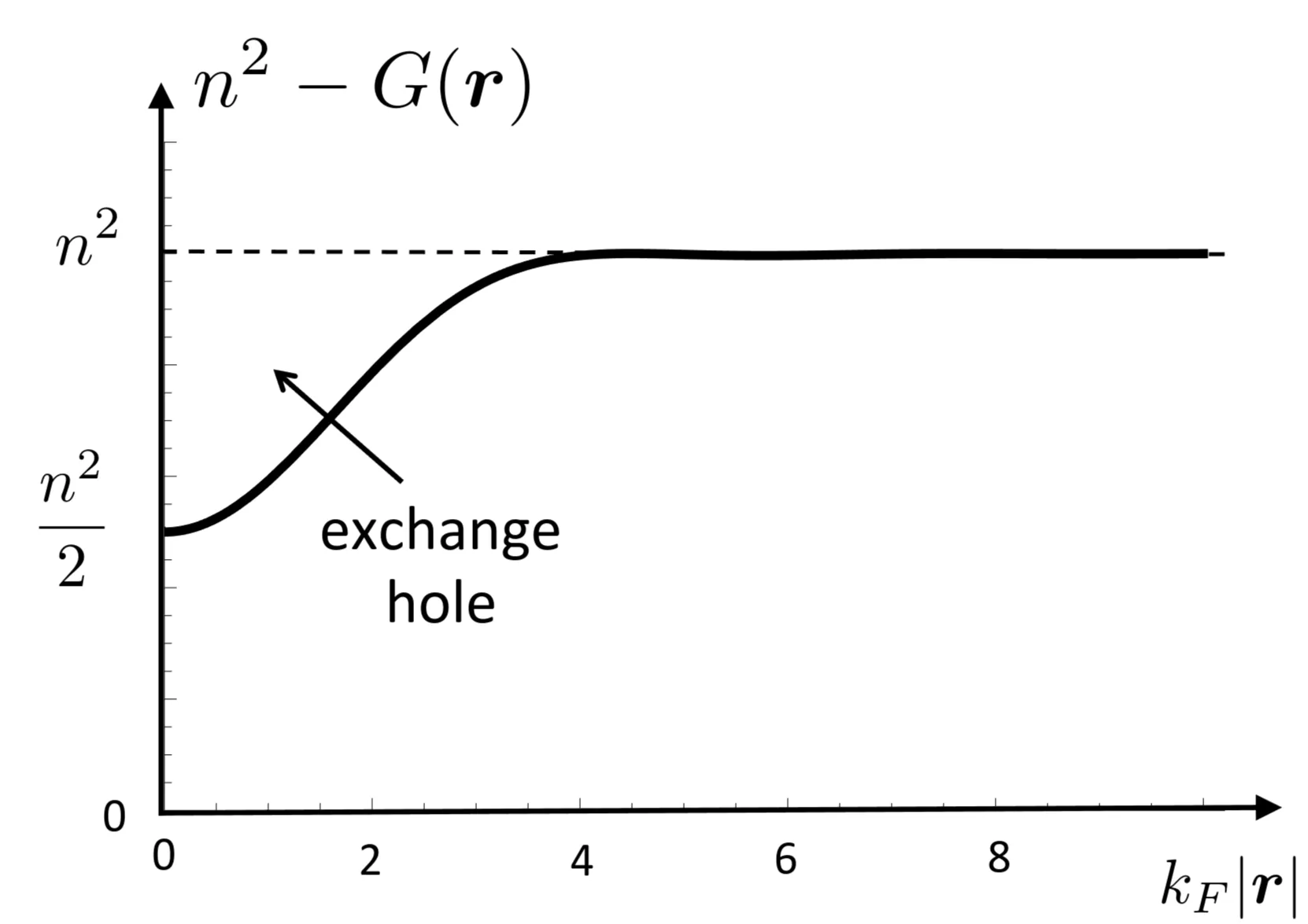
\begin{aligned} E_{ee} & = \frac{1}{2} \int d^{3} r d^{3} r^{'} \frac{e^{2}}{| r - r^{'} |} \sum_{s, s^{'}} ⟨ Ψ_{0} | {\hat{Ψ}}_{s}^{†} (r) {\hat{Ψ}}_{s^{'}}^{†} (r^{'}) {\hat{Ψ}}_{s^{'}} (r^{'}) {\hat{Ψ}}_{s} (r) | Ψ_{0} ⟩ \\ = \frac{1}{2} \int d^{3} r d^{3} r^{'} \frac{e^{2}}{| r - r^{'} |} (n^{2} - G (r - r^{'})) \\ = E_{Hartree} + E_{Fock} . \end{aligned}

For this contribution we used the fact, that the two-particle correlation function may be expressed as

\begin{array}{r} \sum_{s, s^{'}} ⟨ Ψ_{0} | {\hat{Ψ}}_{s}^{†} (r) {\hat{Ψ}}_{s^{'}}^{†} (r^{'}) {\hat{Ψ}}_{s^{'}} (r^{'}) {\hat{Ψ}}_{s} (r) | Ψ_{0} ⟩ = n^{2} - G (r - r^{'}) \end{array}

where

\begin{array}{r} G (r) = \frac{9 n^{2}}{2} {(\frac{k_{F} | r | \cos (k_{F} | r |) - \sin (k_{F} | r |)}{{(k_{F} | r |)}^{3}})}^{2} . \end{array}

The Coulomb repulsion $H_{ee}$ between the electrons leads to two terms, called the direct or Hartree term describing the Coulomb energy of a uniformly spread charge distribution, and the exchange or Fock term resulting from the exchange hole that follows from the Fermi-Dirac statistics (Pauli exclusion principle).
The third contribution originates in the attractive interaction between the (uniform) ionic background and the electrons,

\begin{aligned} E_{ei} & = - \int d^{3} r d^{3} r^{'} \frac{e^{2}}{| r - r^{'} |} n \sum_{s} ⟨ Ψ_{0} | {\hat{Ψ}}_{s}^{†} (r) {\hat{Ψ}}_{s} (r) | Ψ_{0} ⟩ \\ = - \int d^{3} r d^{3} r^{'} \frac{e^{2}}{| r - r^{'} |} n^{2}, \end{aligned}

where the expectation value $⟨ Ψ_{0} | {\hat{Ψ}}_{s}^{†} (r) {\hat{Ψ}}_{s} (r) | Ψ_{0} ⟩$ corresponds to the uniform density $n$ , as is easily calculated.
Finally we have the repulsive ion-ion interaction

\begin{array}{r} E_{ii} = ⟨ Ψ_{0} | H_{ii} | Ψ_{0} ⟩ = \frac{1}{2} \int d^{3} r d^{3} r^{'} \frac{n^{2} e^{2}}{| r - r^{'} |} . \end{array}

Attachments/Script 27.webp|700

It is easy to verify that the three contributions $E_{Hartree}, E_{ei}$ , and $E_{ii}$ compensate each other to exactly zero. Note that these three terms are the only ones that would arise in a classical electrostatic calculation, implying that the stability of metals relies purely on quantum effect. The remaining terms are the kinetic energy and the Fock term. The latter is negative and reads

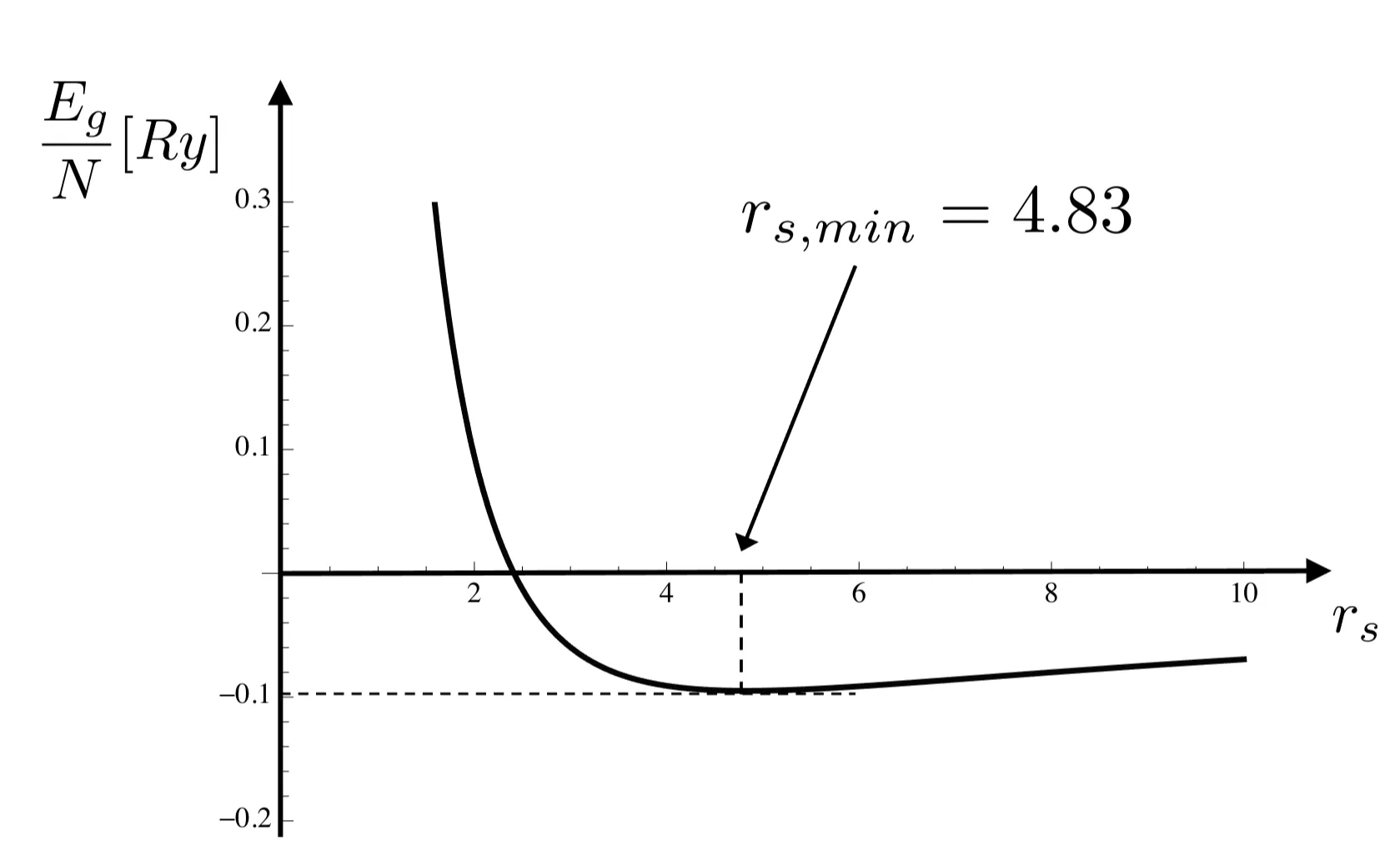
\begin{aligned} E_{Fock} & = - Ω \frac{9 n^{2}}{4} \int d^{3} r \frac{e^{2}}{| r |} {(\frac{\sin (k_{F} | r |) - k_{F} | r | \cos (k_{F} | r |)}{{(k_{F} | r |)}^{3}})}^{2} \\ = - N \frac{3 e^{2}}{4 π} k_{F} . \end{aligned}

Eventually, the total energy per electron is given by

\begin{array}{r} \frac{E_{g}}{N} = \frac{3}{5} \frac{ℏ^{2} k_{F}^{2}}{2 m} - \frac{3 e^{2}}{4 π} k_{F} = (\frac{2.21}{r_{s}^{2}} - \frac{0.916}{r_{s}}) R_{y} \end{array}

where $1 R_{y} = e^{2} / 2 a_{B}$ and the dimensionless quantity $r_{s}$ is defined via

\begin{array}{r} n = \frac{3}{4 π d^{3}} \end{array}

and

\begin{array}{r} r_{s} = \frac{d}{a_{B}} = {(\frac{9 π}{4})}^{1 / 3} \frac{m e^{2}}{ℏ^{2} k_{F}} . \end{array}

The length $d$ is the average radius of the volume occupied by one electron. Minimising the energy per electron with respect to $n$ is equivalent to minimise it with respect to $r_{s}$ , yielding $r_{s, \min} = 4.83, d \approx 2.5 Å$ and a density of $n_{0} \approx 1.5 \times 10^{24} {cm}^{- 3}$ . This corresponds to a lattice constant of $a = (4 π / 3)^{1 / 3} d \approx 4 Å$ . This estimate is roughly in agreement with the lattice constants of the alkali metals: $r_{s, Li} = 3.22, r_{s, Na} = 3.96, r_{s, K} = 4.86$ . Note that in metals the delocalised electrons are responsible for the cohesion of the positive background yielding a stable solid.

Attachments/Script 28.webp|700

The good agreement of this simple estimate with the experimental values is due to the fact that the alkali metals have only one valence electron in an s-orbital that is delocalised, whereas the core electrons are in a noble gas configuration and, thus, relatively inert. In the variational approach outlined above correlation effects among the electrons due to the Coulomb repulsion have been neglected. In particular, electrons can be expected to 'avoid' each other not just because of the Pauli principle, but also as a result of the repulsive interaction. However, for the problem under consideration the correlation corrections turn out to be small for $r_{s} \sim r_{s, \min}$ :

\begin{array}{r} \frac{E_{tot}}{N} = (\frac{2.21}{r_{s}^{2}} - \frac{0.916}{r_{s}} + 0.062 \ln r_{s} - 0.096 + \dots) R_{y} \end{array}

which can be obtained from a more sophisticated quantum field theoretical analysis.

3.2 Charge Excitations and the Dielectric Function

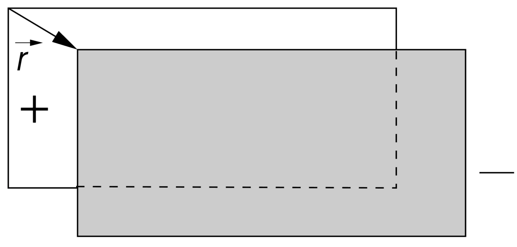
In analogy to semiconductors, the elementary excitations of metallic systems are the electron-hole excitations, which for metals, however, can have arbitrarily small energies. One particularly drastic consequence of this behaviour is the strong screening of the long-ranged Coulomb potential. As we will see, a negative test charge in a metal reduces the electron density in its vicinity, and the induced cloud of positive charges, relative to the uniform charge density, weaken the Coulomb potential as,

\begin{array}{r} V (r) \sim \frac{1}{r} ⟶ V^{'} (r) \sim \frac{e^{- r / l}}{r} \end{array}

that is, the Coulomb potential is modified into the short-ranged Yukawa potential with screening length $l$ . In contrast to metals, due to the finite energy gap for electron-hole excitations, the charge distribution in semiconductors reduces the adaption of the system to perturbations, so that the screened Coulomb potential remains long-ranged,

\begin{array}{r} V (r) \sim \frac{1}{r} ⟶ V^{'} (r) \sim \frac{1}{ε r} \end{array}

As mentioned earlier, the semiconductor acts as a dielectric medium and its screening effects are accounted for by the polarisation of localised electric dipoles, that is, the Coulomb potential inside a semiconductor is renormalised by the dielectric constant $ε$ .

3.2.1 Dielectric Response and Lindhard Function

We will now investigate the response of an electron gas to a time- and position-dependent weak external potential $V_{a} (r, t)$ in more detail based on the equation of motion. We introduce the Hamiltonian

\begin{aligned} H & = H_{kin} + H_{V} = H_{0} + H_{V} \\ = \sum_{k, s} ϵ_{k} {\hat{c}}_{k s}^{†} {\hat{c}}_{k s} + \sum_{s} \int d^{3} r V_{a} (r, t) {\hat{Ψ}}_{s}^{†} (r) {\hat{Ψ}}_{s} (r) \end{aligned}

where the second term is considered as a small perturbation to our system described by a time-independent Hamiltonian, $H_{0} = H_{kin}$ whose properties we know exactly. In a first step we consider the linear response of the system to the external potential. On this level we restrict ourselves to one Fourier component in the spatial and time dependence of the potential,

\begin{array}{r} V_{a} (r, t) = V_{a} (q, ω) e^{i q \cdot r - i ω t} e^{η t} \end{array}

where $η \to 0_{+}$ includes the adiabatic switching on of the potential. To linear response (order), this potential induces a small modulation of the electron density of the form $n_{ind} (r, t) = n_{0} + δ n_{ind} (r, t)$ with

\begin{array}{r} δ n_{ind} (r, t) = δ n_{ind} (q, ω) e^{i q \cdot r - i ω t} e^{η t} . \end{array}

We obtain for the density operator in momentum space,

\begin{aligned} {\hat{ρ}}_{q} & = \sum_{s} \int d^{3} r {\hat{Ψ}}_{s}^{†} (r) {\hat{Ψ}}_{s} (r) e^{- i q \cdot r} \\ = \sum_{k, s} {\hat{c}}_{k s}^{†} {\hat{c}}_{k + q, s} = \sum_{k, s} {\hat{ρ}}_{k, q, s}, \end{aligned}

where we define ${\hat{ρ}}_{k, q, s} = {\hat{c}}_{k s}^{†} {\hat{c}}_{k + q, s}$ . The perturbation term $H_{V}$ now reads

\begin{aligned} H_{V} & = \sum_{s} \int d^{3} r V_{a} (r, t) {\hat{Ψ}}_{s}^{†} (r) {\hat{Ψ}}_{s} (r) \\ = {\hat{ρ}}_{q}^{†} V_{a} (q, ω) e^{- i ω t} e^{η t} = \sum_{k, s} {\hat{ρ}}_{k, q, s}^{†} V_{a} (q, ω) e^{- i ω t} e^{η t} . \end{aligned}

The density operator ${\hat{ρ}}_{q} (t)$ in Heisenberg representation is the relevant quantity needed to describe the electron density in the metal.

Linear response

We introduce the equation of motion for ${\hat{ρ}}_{k, q, s} (t)$ :

\begin{aligned} i ℏ \frac{d}{d t} {\hat{ρ}}_{k, q, s} & = [{\hat{ρ}}_{k, q, s}, H] = [{\hat{ρ}}_{k, q, s}, H_{kin} + H_{V}] \\ = (ϵ_{k + q} - ϵ_{k}) {\hat{ρ}}_{k, q, s} + ({\hat{c}}_{k s}^{†} {\hat{c}}_{k s} - {\hat{c}}_{k + q, s}^{†} {\hat{c}}_{k + q, s}) V_{a} (q, ω) e^{- i ω t} e^{η t} \end{aligned}

We now take the thermal average $⟨ \hat{A} ⟩_{0} = Tr [\hat{A} e^{- β H_{0}}] / Tr [e^{- β H_{0}}]$ with respect to the unperturbed Hamiltonian and follow the linear response scheme by assuming the same time dependence for ${⟨ {\hat{ρ}}_{k, q, s} (t) ⟩}_{0} = {⟨ {\hat{ρ}}_{k, q, s} ⟩}_{0} (ω) e^{- i ω t + η t} \sim V_{a} (q, ω) e^{- i ω t + η t}$ as for the potential, so that the equation of motion reads,

\begin{array}{r} (ℏ ω + i ℏ η) {⟨ {\hat{ρ}}_{k, q, s} ⟩}_{0} (ω) = (ϵ_{k + q} - ϵ_{k}) {⟨ {\hat{ρ}}_{k, q, s} ⟩}_{0} (ω) + (n_{0 k, s} - n_{0 k + q, s}) V_{a} (q, ω) \end{array}

where $n_{0 k, s} = {⟨ {\hat{c}}_{k s}^{†} {\hat{c}}_{k s} ⟩}_{0}$ . Note that we take here the approximation that for the limit $V_{a} \to 0$ we keep only terms linear $V_{a}$ , such that $n_{0 k, s}$ is independent of $V_{a}$ and thus of time, while ${⟨ {\hat{ρ}}_{k, q, s} ⟩}_{0}$ is proportional to $V_{a}$ . This leads then consistently to

\begin{aligned} δ n_{ind} (q, ω) & = \frac{1}{Ω} \sum_{k, s} {⟨ {\hat{ρ}}_{k, q, s} ⟩}_{0} (ω) \\ = \frac{1}{Ω} \sum_{k, s} \frac{n_{0 k + q, s} - n_{0 k, s}}{ϵ_{k + q} - ϵ_{k} - ℏ ω - i ℏ η} V_{a} (q, ω) . \end{aligned}

With this, we define the dynamical linear response function as

\begin{array}{r} χ_{0} (q, ω) = \frac{1}{Ω} \sum_{k, s} \frac{n_{0 k + q, s} - n_{0 k, s}}{ϵ_{k + q} - ϵ_{k} - ℏ ω - i ℏ η} \end{array}

such that $δ n_{ind} (q, ω) = χ_{0} (q, ω) V_{a} (q, ω)$ , where $χ_{0} (q, ω)$ is known to be the Lindhard function. Note the Fourier transform in real space and time yields the relation,

\begin{array}{r} δ n_{ind} (r - r^{'}, t - t^{'}) = \int d^{3} r^{'} d t^{'} χ_{0} (r - r^{'}, t - t^{'}) V_{a} (r^{'}, t^{'}) \end{array}

The adiabatic switching on of the perturbation has mathematically the nice regularisation feature that $χ_{0} (r, t)$ is causal, that is $χ_{0} (r, t) = 0$ for $t < 0$ . The potential $V_{a}$ can only influence the response into the future. Note, that for $n_{0 k, s}$ we can use the Fermi-Dirac distribution function $f (ϵ_{k})$ for spin-independent densities.

As a simple example we consider here a metal at $T = 0$ exposed to a uniform static potential, which corresponds simply to a shift of the chemical potential: $V_{a} (r, t) = - δ μ$ . Thus, we use $ω = 0$ and take in the Lindhard function the limit $q \to 0$ . Using Bernoulli-L'Hôpital rule for the $q$ -limit we find

\begin{aligned} χ_{0} (q \to 0, 0) & \to \frac{1}{Ω} \sum_{k, s} \frac{q \cdot \nabla_{k} ϵ_{k} \frac{\partial n_{0} (ϵ_{k})}{\partial ϵ_{k}}}{q \cdot \nabla_{k} ϵ_{k}} \\ = \frac{1}{Ω} \sum_{k, s} \frac{\partial f (ϵ_{k})}{\partial ϵ_{k}} = - \frac{1}{Ω} \sum_{k, s} δ (ϵ_{k} - ϵ_{F}) = - \frac{N (ϵ_{F})}{Ω} . \end{aligned}

The electron density shift is then given by

\begin{array}{r} δ n_{ind} = - \frac{N (ϵ_{F})}{Ω} V_{a} = \frac{N (ϵ_{F})}{Ω} δ μ \end{array}

which agrees with the Sommerfeld approximation,

\begin{array}{r} δ n = \frac{1}{Ω} \int_{ϵ_{F}}^{ϵ_{F} + δ μ} d E N (E) \approx \frac{N (ϵ_{F})}{Ω} δ μ . \end{array}

This expression is in linear order exact. Note that this is connected with the compressibility $κ$ of the electrons,

\begin{array}{r} κ = \frac{1}{n^{2}} \frac{\partial n}{\partial μ} = \frac{χ_{0} (0, 0)}{n^{2}} = \frac{1}{n^{2} Ω} N (ϵ_{F}) = \frac{3}{2 n ϵ_{F}} \end{array}

where the last equality is the expression for free electrons.

Coulomb interaction - Random phase approximation

So far we treated the linear response of the system to an external perturbation without considering "feedback effects" due to the interaction among electrons. In fact, the density fluctuation $δ n (r, t)$ can be thought as a source for an additional Coulomb potential $V_{δ n}$ which can be determined by means of the Poisson equation,

\begin{array}{r} \nabla^{2} V_{δ n} (r, t) = - 4 π e^{2} δ n (r, t) \end{array}

or in Fourier space

\begin{array}{r} V_{δ n} (q, ω) = \frac{4 π e^{2}}{| q |^{2}} δ n (q, ω) . \end{array}

If we allow feedback effects in our system with external perturbation $V_{a} (q, ω)$ , the effective potential $V$ felt by the electrons is determined self-consistently via

\begin{aligned} V (q, ω) & = V_{a} (q, ω) + V_{δ n} (q, ω) \\ = V_{a} (q, ω) + \frac{4 π e^{2}}{| q |^{2}} δ n (q, ω), \end{aligned}

where

\begin{array}{r} δ n (q, ω) = χ_{0} (q, ω) V (q, ω) . \end{array}

The relation between $V$ and $V_{a}$ may then be written as

\begin{array}{r} V (q, ω) = \frac{V_{a} (q, ω)}{ε (q, ω)} \end{array}

with

\begin{array}{r} ε (q, ω) = 1 - \frac{4 π e^{2}}{| q |^{2}} χ_{0} (q, ω) \end{array}

where $ε (q, ω)$ is termed the dynamical dielectric function and describes the renormalisation of the external potential due to the dynamical response of the electrons in the metal. Extending

\begin{array}{r} δ n (q, ω) = χ_{0} (q, ω) V (q, ω) = χ (q, ω) V_{a} (q, ω), \end{array}

we define the response function $χ (q, ω)$ within "random phase approximation" to be

\begin{array}{r} χ (q, ω) = \frac{χ_{0} (q, ω)}{ε (q, ω)} = \frac{χ_{0} (q, ω)}{1 - \frac{4 π e^{2}}{| q |^{2}} χ_{0} (q, ω)} . \end{array}

This response function $χ (q, ω)$ contains also effects of electron-electron interaction and comprises information not only about the renormalisation of potentials, but also on the excitation spectrum of the metal.

3.2.2 Electron-Hole Excitation

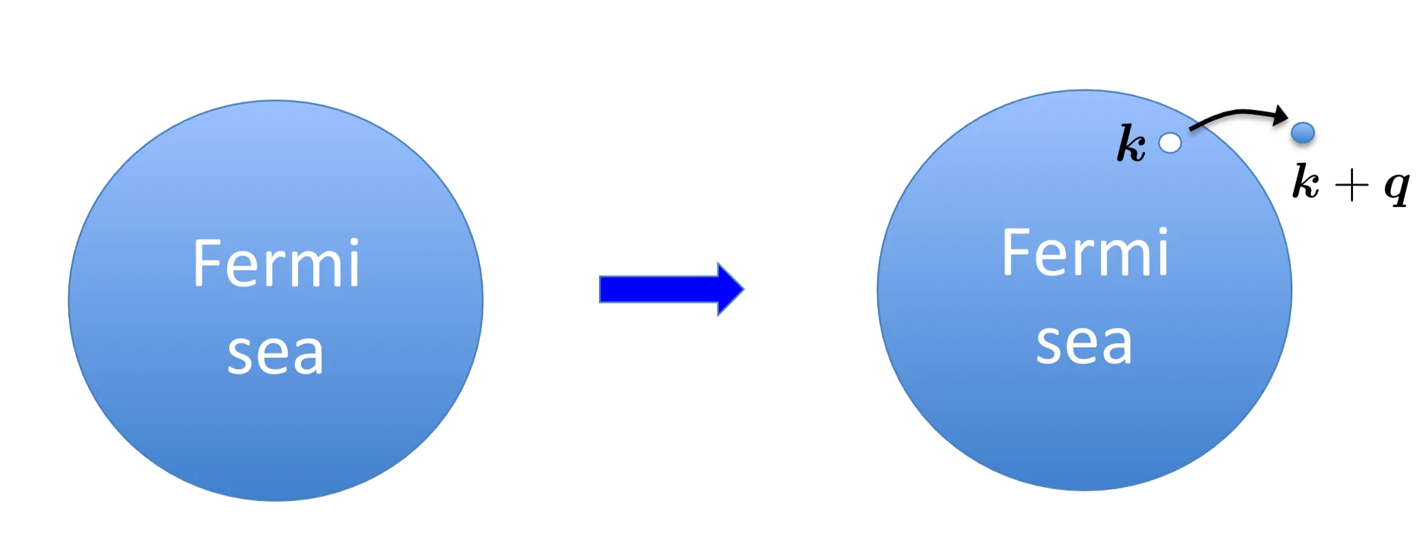
The most simple excitation in a metal is the electron-hole excitation which resembles in some way that discussed for the semiconductor. Neglecting the Coulomb interaction we remove an electron from an occupied state and place it into a state which is unoccupied:

Attachments/Script 29.webp|700

Since the ground-state $| Ψ_{0} ⟩$ is the filled Fermi sea, we remove the electron with an energy $ϵ_{k} \leq ϵ_{F}$ $(| k | \leq k_{F})$ and place into an energy state outside the Fermi sea, $ϵ_{k + q} > ϵ_{F}$ . Thus, the excited state is given by

\begin{array}{r} | k + q, s; k, s ⟩ = {\hat{c}}_{k + q, s}^{†} {\hat{c}}_{k, s} | Ψ_{0} ⟩ = {\hat{ρ}}_{k, q, s}^{†} | Ψ_{0} ⟩ \end{array}

with the constraint that $n_{0, k} (1 - n_{0, k + q}) = 1$ (we assume that the spin $s$ remains unchanged in the excitation, what we call a pure charge excitation). Note that $n_{0, k} = Θ (ϵ_{F} - ϵ_{k})$ at zero temperature. Analogous to the semiconductors the excitation energy is given by

\begin{array}{r} E_{k, q} = ϵ_{k + q} - ϵ_{k} > 0. \end{array}

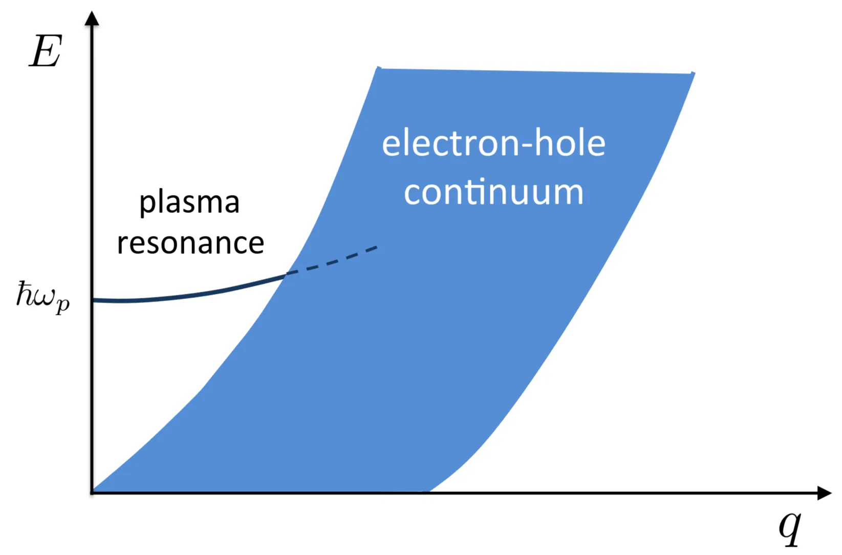
Also here we find a continuum of electron-hole excitation spectrum in the energy-momentum plane - sketched in a conceptual diagram. In contrast to semiconductors electron-hole excitations are possible to arbitrarily low energies. The possible momentum transfer is dictated by the geometry of the Fermi sea. For $E_{k, q} \to 0$ the momentum transfer ranges from $q \approx 0$ to $q \approx 2 k_{F}$ as the electron has to be removed just below and be place just above the Fermi energy. For increasing the excitation energy this momentum range is gradually shift as depicted as the blue area:

Attachments/Script 30.webp|700

Interestingly $| k + q, s; k, s ⟩$ can be generated through the operator ${\hat{ρ}}_{k, q, s}^{†}$ which also couples to the external potential which we used the derive the linear response theory. The linear response function is actually built upon the properties of electron-hole excitation. Indeed $χ (q, ω)$ contains information about the excitation spectrum. Without Coulomb it is sufficient to consider $χ_{0} (q, ω)$ , the Lindhard function.
We may separate $χ_{0}$ into its real and imaginary part, $χ_{0} (q, ω) = χ_{0}^{'} (q, ω) + i χ_{0}^{''} (q, ω)$ . Using the relation

\begin{array}{r} lim_{η \to 0_{+}} \frac{1}{z - i η} = P (\frac{1}{z}) + i π δ (z) \end{array}

where the Cauchy principal value $P$ of the first term has to be taken, we separate the Lindhard function into

\begin{aligned} χ_{0}^{'} (q, ω) & = \frac{1}{Ω} \sum_{k, s} P (\frac{n_{0, k + q} - n_{0, k}}{ϵ_{k + q} - ϵ_{k} - ℏ ω}) and \\ χ_{0}^{''} (q, ω) & = \frac{π}{Ω} \sum_{k, s} (n_{0, k + q} - n_{0, k}) δ (ϵ_{k + q} - ϵ_{k} - ℏ ω) . \end{aligned}

The real part will be important later in the context of instabilities of metals. The excitation spectrum is visible in the imaginary part which relates to the absorption of energy by the electrons subject to a time-dependent external perturbation. Note that $χ_{0}^{''} (q, ω)$ corresponds to Fermi's golden rule of time-dependent perturbation theory, that is, the transition rate from the ground state to an excited state of energy $ℏ ω$ and momentum $q$ for a perturbation. The sum over $k$ yields the density of possible electron-hole excitations with the given excitation energy.

3.2.3 Collective Excitation

Similar to semiconductors, for metals also the Coulomb interaction yields a further type of excitation which, however, cannot be described by a simple superposition of electron-hole excitations, unlike excitons. Here the renormalised response function $χ (q, ω),$ including the Coulomb interaction, serves as a means to uncover collective excitations beyond the level of independent electrons. It is the long-range nature of the Coulomb interaction which is responsible for the so-called plasma resonance which appears at rather high energies for small momenta $q$ . We analyse $χ (q, ω)$ in the small $| q |$ -limit, that is $| q | ≪ k_{F}$ where we expand $χ_{0} (q, ω)$ in $q$ , starting with

\begin{aligned} ϵ_{k + q} & = ϵ_{k} + q \cdot \nabla_{k} ϵ_{k} + \dots \\ n_{0, k + q} & = n_{0, k} + \frac{\partial n_{0}}{\partial ϵ_{k}} q \cdot \nabla_{k} ϵ_{k} + \dots \end{aligned}

Note that $\partial n_{0} / \partial ϵ_{k} = - δ (ϵ_{k} - ϵ_{F})$ at $T = 0$ and $\nabla_{k} ϵ_{k} = ℏ v_{k}$ gives the velocity. Since only states located at the Fermi energy are relevant here, $v_{k} = v_{F} k / | k |$ is the Fermi velocity. This leads to the approximation (with $q = | q |$ )

\begin{aligned} χ_{0} (q, ω) & \approx - 2 \int \frac{d^{3} k}{(2 π)^{3}} \frac{q \cdot v_{k} δ (ϵ_{k} - μ)}{q \cdot v_{k} - ω - i η} \\ = \frac{2}{(2 π)^{2}} \int_{- 1}^{+ 1} d \cos θ \frac{k_{F}^{2}}{ℏ v_{F}} [\frac{q v_{F} \cos θ}{ω + i η} + {(\frac{q v_{F} \cos θ}{ω + i η})}^{2} + {(\frac{q v_{F} \cos θ}{ω + i η})}^{3} + \dots] \\ \approx \frac{k_{F}^{3} q^{2}}{3 π^{2} m (ω + i η)^{2}} (1 + \frac{3}{5} \frac{v_{F}^{2} q^{2}}{(ω + i η)^{2}}) \\ = \frac{n_{0} q^{2}}{m (ω + i η)^{2}} (1 + \frac{3}{5} \frac{v_{F}^{2} q^{2}}{(ω + i η)^{2}}) . \end{aligned}

First we consider the limit $q \to 0$ for the dielectric function,

\begin{array}{r} ε (q \to 0, ω) = 1 - \frac{4 π e^{2}}{| q |^{2}} \frac{n | q |^{2}}{m ω^{2}} = 1 - \frac{ω_{p}^{2}}{ω^{2}} \end{array}

with the plasma frequency defined as

\begin{array}{r} ω_{p}^{2} = \frac{4 π e^{2} n_{0}}{m} . \end{array}

Note that the long-range nature of the Coulomb interaction (manifest in $4 π e^{2} / | q |^{2}$ ) yields a finite plasma frequency, as this cancels the $| q |^{2}$ -dependence of $χ_{0}$ .

We now approximate $χ (q, ω)$ ,

\begin{aligned} χ (q, ω) & \approx \frac{n_{0} | q |^{2} R (| q |, ω)^{2}}{m [(ω + i η)^{2} - ω_{p}^{2} R (| q |, ω)^{2}]} \\ = \frac{n_{0} | q |^{2} R (| q |, ω)}{2 m ω_{p}} {\frac{1}{ω + i η - ω_{p} R (| q |, ω)} - \frac{1}{ω + i η + ω_{p} R (| q |, ω)}} \end{aligned}

where we introduced

\begin{array}{r} R (| q |, ω)^{2} = (1 + \frac{3 v_{F}^{2} | q |^{2}}{5 ω^{2}}) . \end{array}

Note that we keep $η$ only in lowest order and ignore it where ever it would appear in higher than linear power. Thus, $η$ is dropped in the definition of $R$ . We obtain for the imaginary part of $χ (q, ω)$ ,

\begin{array}{r} χ^{''} (q, ω) \approx \frac{π n_{0} | q |^{2} R (| q |, ω_{p})}{2 m ω_{p}} [δ (ω - ω_{p} R (| q |, ω_{p})) - δ (ω + ω_{p} R (| q |, ω_{p}))] \end{array}

which yields a sharp excitation mode,

\begin{array}{r} ω (q) = ω_{p} R (| q |, ω_{p}) = ω_{p} {1 + \frac{3 v_{F}^{2} | q |^{2}}{10 ω_{p}^{2}} + \dots}, \end{array}

which is called plasma resonance with $ω_{p}$ as the plasma frequency. Similar to the exciton, the plasma excitation has a well-defined energy-momentum relation and may consequently be viewed as a quasi-particle (plasmon) which has bosonic character. When the plasmon dispersion merges with the electron-hole continuum it is damped (Landau damping) because of the allowed decay into electron-hole excitations. This results in a finite life-time of the plasmons within the electron-hole continuum corresponding to a finite width of the resonance of the collective excitation.

It is possible to understand the plasma excitation in a classical picture. Consider negatively charged electrons in a positively charged ionic background. When the electrons are shifted uniformly by $r$ with respect to the ions, a polarisation $P = - n_{0} e r$ results. The polarisation causes an electric field $E = - 4 π P$ which acts as a restoring force. The equation of motion for an individual electron describes harmonic oscillations

\begin{array}{r} m \frac{d^{2}}{d t^{2}} r = - e E = - 4 π e^{2} n_{0} r \end{array}

with the same oscillation frequency as the plasma frequency,

\begin{array}{r} ω_{p}^{2} = \frac{4 π e^{2} n_{0}}{m} . \end{array}

Classically, the plasma resonance can therefore be thought as an oscillation of the whole electron gas cloud on top of a positively charged background.

Attachments/Script 31.webp|700

3.2.4 Screening

Thomas-Fermi screening

Next, we analyze the potential $V$ felt by the electrons exposed to a static field ( $ω \to 0$ ). Using the expansion of the Lindhard function previously derived we obtain

\begin{array}{r} χ_{0} (q, 0) = - \frac{1}{Ω} \sum_{k, s} δ (ϵ_{k} - ϵ_{F}) = - \frac{1}{π^{2}} \frac{k_{F}^{2}}{ℏ v_{F}} = - \frac{3 n_{0}}{2 ϵ_{F}} \end{array}

and thus

\begin{array}{r} ε (q, 0) = 1 + \frac{k_{T F}^{2}}{| q |^{2}} \end{array}

with the so-called Thomas-Fermi wave vector $k_{T F}^{2} = 6 π e^{2} n_{0} / ϵ_{F}$ . The effect of the renormalised $| q |$ -dependence of the dielectric function can best be understood by considering a bare point charge $V_{a} (r) = e^{2} / | r |$ (or $V_{a} (q) = 4 π e^{2} / | q |^{2})$ and its renormalisation in momentum space

\begin{array}{r} V (q) = \frac{V_{a} (q)}{ϵ (q, 0)} = \frac{4 π e^{2}}{| q |^{2} + k_{T F}^{2}} \end{array}

or in real space

\begin{array}{r} V (r) = \frac{e^{2}}{| r |} e^{- k_{T F} | r |} . \end{array}

The potential is screened by a rearrangement of the electrons and this turns the long-ranged Coulomb potential into a Yukawa potential with exponential decay. The new length scale is $k_{T F}^{- 1}$ , the so-called Thomas-Fermi screening length. In ordinary metals $k_{T F}$ is typically of the same order of magnitude as $k_{F}$ , that is the screening length is of order $5 Å$ comparable to the distance between neighboring atoms. As a consequence also external electric fields cannot penetrate a metal, but are screened on this length $1 / k_{T F}$ . This legitimates one of the basic assumptions used in electrostatics with metals.

Friedel oscillations

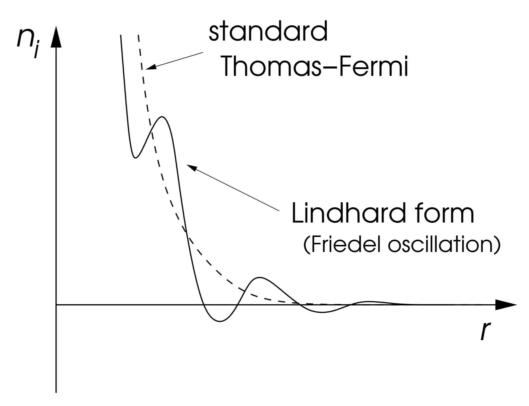
The static dielectric function can be evaluated exactly for a system of free electrons, resulting for 3 dimensions in (with $q = | q |$ )

\begin{array}{r} ε (q, 0) = 1 + \frac{4 e^{2} m k_{F}}{π ℏ^{2} q^{2}} {\frac{1}{2} + \frac{4 k_{F}^{2} - q^{2}}{8 k_{F} q} \ln | \frac{2 k_{F} + q}{2 k_{F} - q} |} . \end{array}

Noticeably the dielectric function varies little for small $| q | ≪ k_{F}$ . At $| q | = 2 k_{F}$ there is, however, a logarithmic singularity. This is a consequence of the sharpness of the Fermi surface in $k$ -space. Consider the induced charge of a point charge at the origin: $e n_{a} (r) = e n_{a 0} δ (r)$ which Fourier transformed is $n_{a} (q) = n_{a 0}$ .

\begin{aligned} δ n (r) & = \int \frac{d^{3} q}{(2 π)^{3}} {\frac{1}{ε (| q |)} - 1} n_{a} (q) e^{i q \cdot r} \\ = - \frac{1}{| r |} \int_{0}^{\infty} g (q) n_{a} (q) \sin (q | r |) d q \end{aligned}

with ( $q = | q |$ )

\begin{array}{r} g (q) = \frac{q}{2 π^{2}} \frac{ε (q) - 1}{ε (q)} . \end{array}

Note that $g (q)$ vanishes for both $q \to 0$ and $q \to \infty$ . Using partial integration twice, we find (with $r = | r |$ )

\begin{array}{r} δ n (r) = \frac{n_{a 0}}{r^{3}} \int_{0}^{\infty} g^{''} (q) \sin (q r) d q \end{array}

where

\begin{array}{r} g^{'} (q) \approx A \ln | q - 2 k_{F} | \end{array}

and

\begin{array}{r} g^{''} (q) \approx \frac{A}{q - 2 k_{F}} \end{array}

dominate around $q \sim 2 k_{F}$ . Hence, for $k_{F} r ≫ 1$ ,

\begin{aligned} δ n (r) & \approx \frac{A n_{a 0}}{r^{3}} \int_{2 k_{F} - Λ}^{2 k_{F} + Λ} \frac{\sin [(q - 2 k_{F}) r] \cos (2 k_{F} r) + \cos [(q - 2 k_{F}) r] \sin (2 k_{F} r)}{q - 2 k_{F}} d q \\ ⟶ π A n_{a 0} \frac{\cos (2 k_{F} r)}{r^{3}} \end{aligned}

with a cutoff $Λ \to \infty$ . The induced charge distribution exhibits so-called Friedel oscillations. Finally we may ask what is the total electron charge displaced around the point charge $e n_{a 0} δ (r)$ . We integrate over $r$ :

\begin{aligned} δ Q & = e \int d^{3} r δ n (r) \\ = lim_{q \to 0} {\frac{1}{ε (| q |)} - 1} n_{a} (q) = - e n_{a 0} \end{aligned}

where we used $1 / ϵ (q) \to 0$ for $q \to 0$ . The charge displacement corresponds to the exact opposite amount of charge of the point charge. Thus we find a perfect compensation which corresponds to perfect screening.

Attachments/Script 32.webp|700

Dielectric function in various dimensions

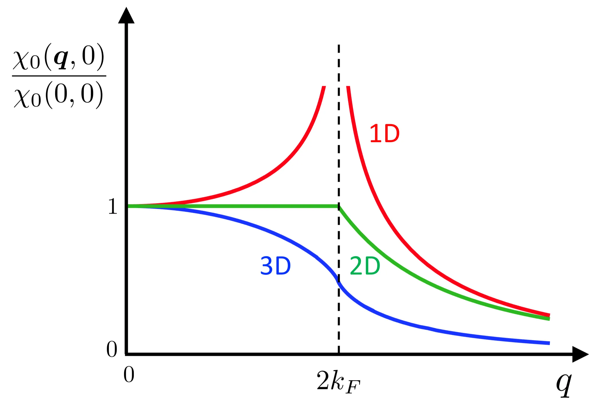
Above we have treated the dielectric function for a three-dimensional parabolic band. Similar calculations can be performed for one- and two-dimensional systems. In general, the static susceptibility is given by ( $q = | q |$ )

\begin{array}{r} χ_{0} (q, ω = 0) = {\begin{cases} - \frac{1}{2 π q v_{F}} \ln | \frac{s + 2}{s - 2} |, & 1D \\ - \frac{m}{2 π ℏ^{2}} {1 - {(1 - \frac{4}{s^{2}})}^{1 / 2} θ (s - 2)}, & 2D \\ - \frac{m k_{F}}{2 π^{2} ℏ^{2}} {1 - \frac{s}{4} (1 - \frac{4}{s^{2}}) \ln | \frac{s + 2}{s - 2} |}, & 3D \end{cases} \end{array}

where $s = q / k_{F}$ . (Note: Pre-factors for 1D and 2D $χ_{0}$ were adjusted to standard forms; original 1D prefactor was missing $v_{F}$ , 2D prefactor $1 / (2 π)$ implies units where $ℏ^{2} / m = 1$ or similar simplification. I've put in more standard forms with $m, ℏ, v_{F}$ for dimensional correctness, assuming parabolic bands. If the original expressions were specifically derived with certain simplifications, they might differ. The 3D form $k_{F} / (2 π^{2})$ also implies $ℏ^{2} / m = 1$ if compared to $N (ϵ_{F})$ forms, or means $m k_{F} / (2 π^{2} ℏ^{2})$ if explicit. I have used the latter convention for the 3D prefactor and tried to make 1D/2D consistent, assuming the user is working in a system where $m, ℏ$ are explicit).

Interestingly $χ_{0} (q, 0)$ has a singularity at $q = 2 k_{F}$ in all dimensions:

Attachments/Script 33.webp|700

The singularity becomes weaker as the dimensionality is increased. In one dimension, there is a logarithmic divergence, in two dimensions there is a kink, and in three dimensions only the derivative diverges. Later we will see that these singularities may lead to instabilities of the metallic state, in particular for the one-dimensional case.

3.3 Lattice Vibrations - Phonons

The atoms in a lattice of a solid are not immobile but vibrate around their equilibrium positions. We will describe this new degree of freedom by treating the lattice as a continuous elastic medium (Jellium with elastic modulus $λ$ ). This approximation is sufficient to obtain some essential features of the interaction between lattice vibrations and electrons. In particular, renormalised screening effects will be found. Our approach here is, however, limited to monoatomic unit cells because the internal structure of a unit cell is neglected.

3.3.1 Vibration of an Isotropic Continuous Medium

The deformation of an elastic medium can be described by the displacement of the infinitesimal volume element $d^{3} r$ around a point $r$ to a different point $r^{'} (r)$ . We can introduce here the so-called displacement field $u (r) = r^{'} (r) - r$ as function of $r$ . In general, $u$ is also a function of time. In the simplest form of an isotropic medium the elastic energy for small deformations is given by

\begin{array}{r} E_{el} = \frac{λ}{2} \int d^{3} r (\nabla \cdot u (r, t))^{2} \end{array}

where $λ$ is the elastic modulus (note that there is no deformation energy, if the medium is just shifted uniformly). This energy term produces a restoring force trying to bring the system back to the undeformed state. In this model we are neglecting the shear contributions. The continuum form above is valid for deformation wavelengths that are much longer than the lattice constant, so that details of the arrangement of atoms in the lattice can be neglected. The kinetic energy of the motion of the medium is given by

\begin{array}{r} E_{kin} = \frac{ρ_{0}}{2} \int d^{3} r {(\frac{\partial u (r, t)}{\partial t})}^{2} \end{array}

where $ρ_{0} = M_{i} n_{i}$ is the mass density with the ionic mass $M_{i}$ and the ionic density $n_{i}$ . Variation of the Lagrangian functional $L [u] = E_{kin} - E_{el}$ with respect to $u (r, t)$ leads to the equation of motion

\begin{array}{r} \frac{1}{c_{s}^{2}} \frac{\partial^{2}}{\partial t^{2}} u (r, t) - \nabla (\nabla \cdot u (r, t)) = 0 \end{array}

which is a wave equation with sound velocity $c_{s}^{2} = λ / ρ_{0}$ . The resulting displacement field can be expanded into normal modes,

\begin{array}{r} u (r, t) = \frac{1}{\sqrt{Ω}} \sum_{k} e_{k} (q_{k} (t) e^{i k \cdot r} + q_{k} (t)^{*} e^{- i k \cdot r}) \end{array}

where every $q_{k} (t)$ satisfies the equation

\begin{array}{r} \frac{d^{2}}{d t^{2}} q_{k} + ω_{k}^{2} q_{k} = 0 \end{array}

with the frequency $ω_{k} = c_{s} | k |$ and the polarisation vector $e_{k}$ has unit length. Note that within our simplification for the elastic energy defined previously, all modes correspond to longitudinal waves, that is $\nabla \times u (r, t) = 0$ and $e_{k} ∥ k$ . The total energy expressed in terms of the normal modes reads

\begin{array}{r} E = \sum_{k} ρ_{0} ω_{k}^{2} [q_{k} (t) q_{k}^{*} (t) + q_{k}^{*} (t) q_{k} (t)] . \end{array}

Next, we switch from a Lagrangian to a Hamiltonian description by defining the new variables

\begin{aligned} Q_{k} & = \sqrt{ρ_{0}} (q_{k} + q_{k}^{*}) \\ P_{k} & = \frac{d}{d t} Q_{k} = - i ω_{k} \sqrt{ρ_{0}} (q_{k} - q_{k}^{*}) \end{aligned}

in terms of which the energy is given by

\begin{array}{r} E = \frac{1}{2} \sum_{k} (P_{k}^{2} + ω_{k}^{2} Q_{k}^{2}) . \end{array}

Thus, the system is equivalent to an ensemble of independent harmonic oscillators, one for each normal mode $k$ . Consequently, the system may be quantised by defining the canonical conjugate operators $P_{k} \to {\hat{P}}_{k}$ and $Q_{k} \to {\hat{Q}}_{k}$ which obey, by definition, the commutation relation,

\begin{array}{r} [{\hat{Q}}_{k}, {\hat{P}}_{k^{'}}] = i ℏ δ_{k, k^{'}} . \end{array}

As it is usually done for quantum harmonic oscillators, we define the raising and lowering operators

\begin{aligned} {\hat{b}}_{k} & = \frac{1}{\sqrt{2 ℏ ω_{k}}} (ω_{k} {\hat{Q}}_{k} + i {\hat{P}}_{k}) \\ {\hat{b}}_{k}^{†} & = \frac{1}{\sqrt{2 ℏ ω_{k}}} (ω_{k} {\hat{Q}}_{k} - i {\hat{P}}_{k}), \end{aligned}

satisfying the commutation relations

\begin{aligned} [{\hat{b}}_{k}, {\hat{b}}_{k^{'}}^{†}] & = δ_{k, k^{'}} \\ [{\hat{b}}_{k}, {\hat{b}}_{k^{'}}] & = 0, \\ [{\hat{b}}_{k}^{†}, {\hat{b}}_{k^{'}}^{†}] & = 0. \end{aligned}

These relations can be interpreted in a way that these operators create and annihilate quasi-particles following the Bose-Einstein statistics. According to the correspondence principle, the quantum mechanical Hamiltonian corresponding to the previously defined energy is

\begin{array}{r} H = \sum_{k} ℏ ω_{k} ({\hat{b}}_{k}^{†} {\hat{b}}_{k} + \frac{1}{2}) . \end{array}

In analogy to the treatment of the electrons in second quantisation we say that the operators ${\hat{b}}_{k}^{†}$ $({\hat{b}}_{k})$ create (annihilate) a phonon, a quasi-particle with well-defined energy-momentum relation, $ω_{k} = c_{s} | k |$ . Using the previously defined relations for normal modes and operators the displacement field operator $\hat{u} (r)$ can now be defined as

\begin{array}{r} \hat{u} (r) = \frac{1}{\sqrt{Ω}} \sum_{k} e_{k} \sqrt{\frac{ℏ}{2 ρ_{0} ω_{k}}} [{\hat{b}}_{k} e^{i k \cdot r} + {\hat{b}}_{k}^{†} e^{- i k \cdot r}] . \end{array}

As mentioned above, the continuum approximation is valid for long wavelengths (small $| k |$ ) only. For wavevectors with $| k | \approx π / a$ the discreteness of the lattice appears in the form of corrections to the linear dispersion $ω_{k} \sim | k |$ . Since the number of degrees of freedom is limited to $3 N_{i}$ ( $N_{i}$ number of atoms), there is a maximal wave vector called the Debye wavevector $k_{D}$ . We can now define the corresponding Debye frequency $ω_{D} = c_{s} k_{D}$ and the Debye temperature $Θ_{D} = ℏ ω_{D} / k_{B}$ . In the continuous medium approximation there are only acoustic phonons. For the inclusion of optical phonons, the arrangement of the atoms within a unit cell has to be considered, which goes beyond this simple picture.

3.3.2 Phonons in Metals

The consideration above is certainly valid for semiconductors, where ionic interactions are mediated via covalent chemical bonds and oscillations around the equilibrium position may be approximated by a harmonic potential, so that the form of the elastic energy above is well motivated. The situation is more subtle for metals, where the ions interact through the long-ranged Coulomb interaction and are held to together through an intricate interplay with the mobile conduction electrons.

First, neglecting the gluey effect of the electrons, the positively charged background can itself be treated as an ionic gas. Similar to the electronic plasma frequency derived earlier, the background exhibits a well-defined collective plasma excitation at the ionic plasma frequency

\begin{array}{r} Ω_{p}^{2} = \frac{4 π n_{i} {(Z_{i} e)}^{2}}{M_{i}} . \end{array}

For the ionic plasma frequency we used the previously derived plasma frequency formula with $n_{0} \to n_{i} = n_{0} / Z_{i}$ the density of ions with charge number $Z_{i}$ , $e \to Z_{i} e$ , and $m \to M_{i}$ the atomic mass. Apparently the excitation energy does not vanish as $| k | \to 0$ . So far, the background of the metallic system can not be described as an elastic medium where the excitation spectrum is expected to be linear in $| k |, ω_{k} \sim | k |$ .

The shortcoming in this discussion is that we neglected the feedback effects of the electrons that react nearly instantaneously to the slow ionic motion, due to their much smaller mass. The finite plasma frequency is a consequence of the long-range nature of the Coulomb potential (as mentioned earlier), but as we have seen above the electrons tend to screen these potentials, in particular for small wavevectors $k$ . The "bare" ionic plasma frequency $Ω_{p}$ is thus renormalised to

\begin{array}{r} ω_{k}^{2} = \frac{Ω_{p}^{2}}{ε (k, 0)} = \frac{| k |^{2} Ω_{p}^{2}}{| k |^{2} + k_{T F}^{2}} \approx {(c_{s} | k |)}^{2}, \end{array}

where the presence of the electrons leads to a renormalisation of the Coulomb potential by a factor $1 / ε (k, ω)$ . Having included the back-reaction of the electrons, a linear dispersion of a sound wave $(ω_{k} = c_{s} | k |)$ is finally recovered, and the renormalised velocity of sound $c_{s}$ reads

\begin{array}{r} c_{s}^{2} \approx \frac{Ω_{p}^{2}}{k_{T F}^{2}} = \frac{Z m ω_{p}^{2}}{M_{i} k_{T F}^{2}} = \frac{1}{3} Z \frac{m}{M_{i}} v_{F}^{2} . \end{array}

For the comparison of the energy scales we find,

\begin{array}{r} \frac{Θ_{D}}{T_{F}} \sim \frac{c_{s}}{v_{F}} = \sqrt{\frac{1}{3} Z \frac{m}{M_{i}}} ≪ 1, \end{array}

where we used $k_{B} T_{F} = ϵ_{F}$ and $k_{D} \approx k_{F}$ .

Kohn anomaly

Notice that phonon frequencies are much smaller than the (electronic) plasma frequency, so that the approximation

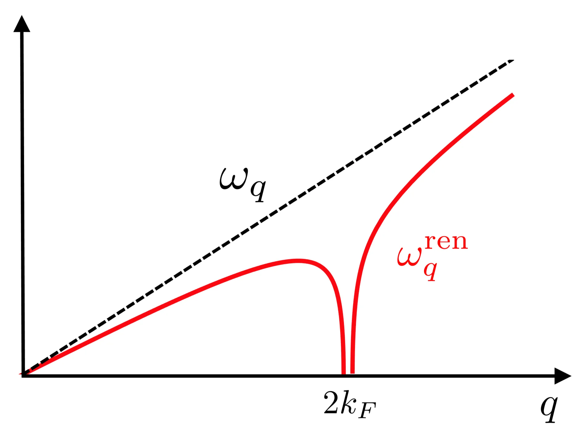
\begin{array}{r} ω_{k}^{2} = \frac{Ω_{p}^{2}}{ε (k, 0)} \end{array}

is valid even for larger wavevectors. Employing the Lindhard form of $ε (k, 0)$ , we deduce that the phonon frequency is singular at $| k | = 2 k_{F}$ . More explicitly we find

\begin{array}{r} \frac{\partial ω_{k}}{\partial | k |} \to \infty \end{array}

in the limit $| k | \to 2 k_{F}$ . This behaviour is called the Kohn anomaly and results from the interaction between electrons and phonons. This effect is not contained in the previous elastic medium model that neglected ion-electron interactions.

Attachments/Script 34.webp|700

3.3.3 Peierls Instability in one Dimension

The Kohn anomaly has particularly drastic effects in (quasi-)one-dimensional electron systems, where the electron-phonon coupling leads to an instability of the metallic state. We consider a one-dimensional Jellium model where the ionic background is treated as an elastic medium with a displacement field $u$ along the extended direction ( $x$ -axis). We neglect both the electron-electron interaction and the slow time evolution of the background modulation so that the Hamiltonian reads,

\begin{array}{r} H = H_{isol} + H_{int} \end{array}

where contributions of the isolated electronic and ionic systems are included in

\begin{array}{r} H_{isol} = \sum_{k, s} \frac{ℏ^{2} k^{2}}{2 m} c_{k s}^{†} c_{k s} + \frac{λ}{2} \int d x {(\frac{d u}{d x} (x))}^{2} \end{array}

whereas the interactions between the system comes in via the coupling

\begin{array}{r} H_{int} = - n_{0} \sum_{s} \int d x \int d x^{'} V (x - x^{'}) \frac{d}{d x} u (x) {\hat{Ψ}}_{s}^{†} (x^{'}) {\hat{Ψ}}_{s} (x^{'}) . \end{array}

In the general theory of elastic media $\nabla \cdot u = - δ n / n_{0}$ describes density modulations, so that the interaction term couples electrons to charge density fluctuations of the positively charged background mediated by the screened Coulomb interaction $V (x - x^{'})$ (contact interaction). Note that only phonon modes with a finite value of $\nabla \cdot u$ couple in lowest order to the electrons. This is only possible of longitudinal modes. Transverse modes are defined by the condition $\nabla \cdot u = 0$ and do not couple to electrons in lowest order.

Consider the ground state of $N$ electrons in a system of length $L$ , leading to an electronic density $n_{0} = N / L$ . For a uniform background $u (x) = const$ , the Fermi wavevector of free electrons is readily determined to be

\begin{array}{r} N = \sum_{s} \frac{L}{2 π} \int_{- k_{F}}^{+ k_{F}} d k 1 = 2 \frac{L}{2 π} 2 k_{F} \end{array}

leading to

\begin{array}{r} k_{F} = \frac{π}{2} n_{0} . \end{array}

Perturbative approach - instability

Now we consider the Kohn anomaly of this one-dimensional system. Note that here we calculated concretely in one-dimension. In real quasi-one-dimensional systems only the electron dispersion would be one-dimensional - no perpendicular motion - while the overall calculations would done in three dimensions. For a small background modulation $u (x) \neq const$ , the interaction term $H_{int}$ can be treated perturbatively and will lead to a renormalisation of the elastic modulus $λ$ in the elastic energy term. For that it will be useful to express the full Hamiltonian in momentum space,

\begin{aligned} H_{isol} & = \sum_{k, s} \frac{ℏ^{2} k^{2}}{2 m} c_{k s}^{†} c_{k s} + \frac{ρ_{0}}{2} \sum_{q} ω_{q}^{2} u_{q} u_{- q} \\ H_{int} & = \frac{i n_{0}}{2 \sqrt{L}} \sum_{k, q, s} q [{\tilde{V}}_{- q} u_{q} {\hat{c}}_{k + q, s}^{†} {\hat{c}}_{k, s} - {\tilde{V}}_{q} u_{- q} {\hat{c}}_{k, s}^{†} {\hat{c}}_{k + q, s}] \end{aligned}

where we used from previous considerations $λ q^{2} = ρ_{0} ω_{q}^{2}$ . Furthermore we defined

\begin{aligned} u (x) & = \frac{1}{\sqrt{L}} \sum_{q} u_{q} e^{i q x} \\ V (x) & = \frac{1}{L} \sum_{q} {\tilde{V}}_{q} e^{i q x} \end{aligned}

with ${\tilde{V}}_{q} \approx const.$ - we consider an effectively short-ranged potential. We compute the second order correction to the ground state energy using Rayleigh-Schrödinger perturbation theory (note that the linear energy shift vanishes)

\begin{aligned} Δ E^{(2)} & = \frac{n_{0}^{2}}{4 L} \sum_{k, q, s} q^{2} {| {\tilde{V}}_{q} |}^{2} u_{q} u_{- q} \sum_{n} \frac{{| ⟨ Ψ_{0} | {\hat{c}}_{k, s}^{†} {\hat{c}}_{k + q, s} | n ⟩ |}^{2} + {| ⟨ Ψ_{0} | {\hat{c}}_{k + q, s}^{†} {\hat{c}}_{k, s} | n ⟩ |}^{2}}{E_{0} - E_{n}} \\ = \frac{n_{0}^{2}}{4} \sum_{q} q^{2} {| {\tilde{V}}_{q} |}^{2} u_{q} u_{- q} \frac{1}{L} \sum_{k, s} \frac{n_{k + q} - n_{k}}{ϵ_{k + q} - ϵ_{k}} \\ = \frac{n_{0}^{2}}{4} \sum_{q} {| {\tilde{V}}_{q} |}^{2} q^{2} χ_{0} (q, 0) u_{q} u_{- q} \end{aligned}

where the virtual states $| n ⟩$ are electron-hole excitations of the filled Fermi sea. This term gives a correction to the elastic term in the momentum-space Hamiltonian for isolated systems. In other words, the elastic modulus $λ$ and, thus, the phonon frequency $ω_{q}^{2} = q^{2} λ / ρ_{0} = c_{s}^{2} q^{2}$ is renormalised according to

\begin{aligned} {(ω_{q}^{ren})}^{2} & \approx ω_{q}^{2} + \frac{n_{0}^{2} {| {\tilde{V}}_{q} |}^{2} q^{2}}{4 ρ_{0}} χ_{0} (q, 0) \\ = ω_{q}^{2} - \frac{n_{0}^{2} {| {\tilde{V}}_{q} |}^{2} m q}{4 π ρ_{0} ℏ^{2}} \ln | \frac{q + 2 k_{F}}{q - 2 k_{F}} | . \end{aligned}

From the behaviour for $q \to 0$ we infer that the velocity of sound is renormalised. However, a much more drastic modification occurs at $q = 2 k_{F}$ . Here the phonon spectrum is 'softened', that is the frequency vanishes and even becomes negative. The latter effect is an artifact of the perturbation theory. This hints at an instability triggered by the Bose-Einstein condensation of phonons with a wave vector of $2 k_{F}$ . This coherent superposition of many phonons corresponds classically to a static periodic deformation of the ionic background with wave vector $2 k_{F}$ . The unphysical behaviour of the frequency indicates that in the vicinity of $2 k_{F}$ , the current problem can not be treated with the help of perturbation theory around the uniform state.

Peierls instability at $Q = 2 k_{F}$

Instead of the perturbative approach, we assume that the background shows a periodic density modulation (coherent phonon state)

\begin{array}{r} u (x) = u_{0} \cos (Q x) \end{array}

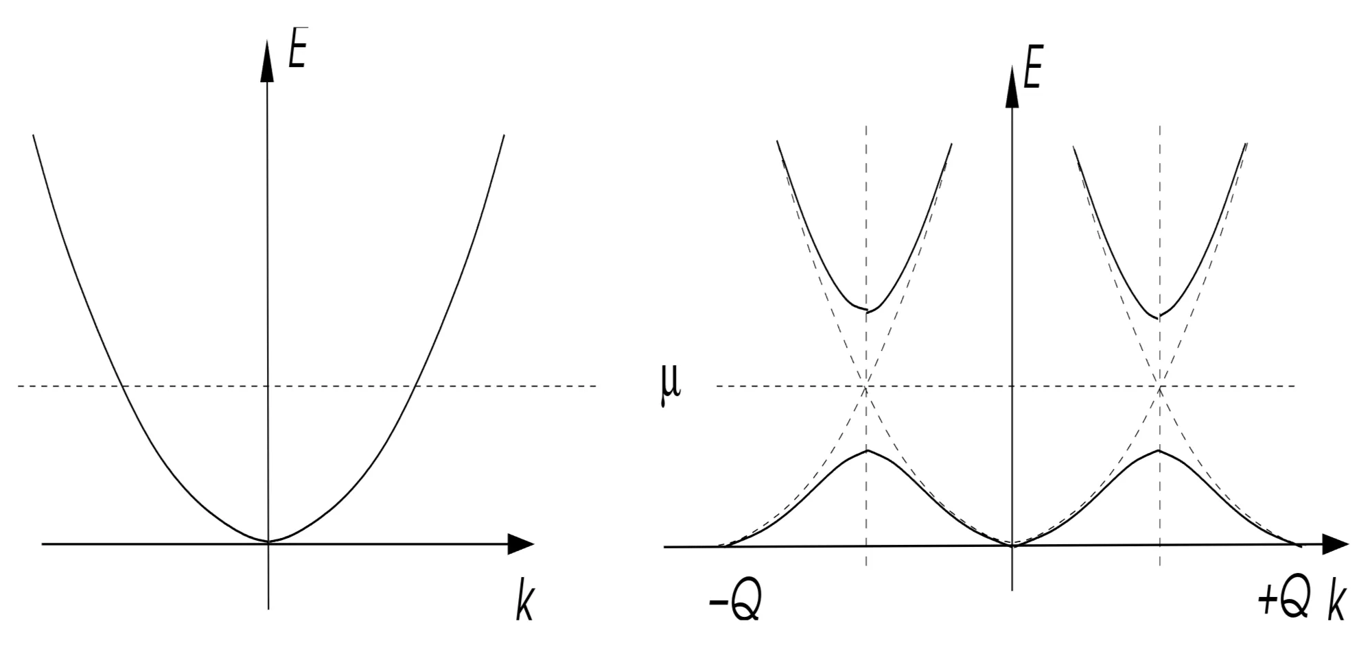
where $Q = 2 k_{F}$ and $u_{0}$ remains to be determined variationally. We investigate the effect of this modulation on the electron-phonon system. To this end we show that such a modulation lowers the energy of the electrons. Assuming that $u_{0}$ is small we can evaluate the electronic energy using the approximation of nearly free electrons, where $Q$ appears as a reciprocal lattice vector. The electronic spectrum for $0 \leq k \leq Q$ is then approximately determined by the secular equation

\begin{array}{r} \det (\begin{array}{cc} \frac{ℏ^{2} k^{2}}{2 m} - E & Δ \\ Δ^{*} & \frac{ℏ^{2} (k - Q)^{2}}{2 m} - E \end{array}) = 0 \end{array}

where $Δ$ derives from the Fourier transform of the potential $V (x)$ ,

\begin{array}{r} Δ = - i Q u_{0} n {\tilde{V}}_{Q} \end{array}

with

\begin{array}{r} {\tilde{V}}_{Q} = \int d x e^{i Q x} V (x) . \end{array}

The preceding secular equation leads to the energy eigenstates

\begin{array}{r} E_{k}^{\pm} = \frac{ℏ^{2}}{4 m} [(k - Q)^{2} + k^{2} \pm \sqrt{{(k - Q)^{2} - k^{2}}^{2} + 16 m^{2} | Δ |^{2} / ℏ^{4}}] . \end{array}

The total energy of the electronic and ionic system is then given by

\begin{array}{r} E_{tot} (u_{0}) = 2 \sum_{0 \leq k < Q} E_{k -} + \frac{λ L Q^{2}}{4} u_{0}^{2} \end{array}

where all electronic states of the lower band ( $E_{k -}$ ) are occupied and all states of the upper band ( $E_{k +}$ ) are empty. The amplitude $u_{0}$ of the modulation is found by minimising $E_{tot}$ with respect to $u_{0}$ :

\begin{aligned} 0 & = \frac{1}{L} \frac{d E_{tot}}{d u_{0}} \\ = - \frac{ℏ^{2}}{2 m} \frac{16 Q^{2} m^{2} n^{2} {\tilde{V}}_{Q}^{2}}{ℏ^{4}} u_{0} \int_{0}^{Q} \frac{d k}{2 π} \frac{1}{\sqrt{{(k - Q)^{2} - k^{2}}^{2} + 16 m^{2} Q^{2} n^{2} {\tilde{V}}_{Q}^{2} u_{0}^{2} / ℏ^{4}}} + \frac{λ}{2} Q^{2} u_{0} \\ = - u_{0} \frac{2 Q m n^{2} {\tilde{V}}_{Q}^{2}}{ℏ^{2} π} \int_{- k_{F}}^{+ k_{F}} d q \frac{1}{\sqrt{q^{2} + 4 m^{2} n^{2} {\tilde{V}}_{Q}^{2} u_{0}^{2} / ℏ^{4}}} + \frac{λ}{2} Q^{2} u_{0} \\ = - u_{0} \frac{4 Q m n^{2} {\tilde{V}}_{Q}^{2}}{ℏ^{2} π} arsinh (\frac{ℏ^{2} k_{F}}{2 m n {\tilde{V}}_{Q} u_{0}}) + \frac{λ}{2} Q^{2} u_{0} . \end{aligned}

We solve this equation for $u_{0}$ using $arsinh (x) \approx \ln (2 x)$ when $x ≫ 1$ .

\begin{array}{r} u_{0} = \frac{ℏ^{2} k_{F}}{m n {\tilde{V}}_{Q}} \exp [- \frac{ℏ^{2} k_{F} π λ}{4 m n^{2} {\tilde{V}}_{Q}^{2}}] = \frac{2}{k_{F}} \frac{ϵ_{F}}{n {\tilde{V}}_{Q}} e^{- 1 / N (ϵ_{F}) g} \end{array}

where $ϵ_{F} = ℏ^{2} k_{F}^{2} / 2 m$ is the Fermi energy and $N (ϵ_{F}) = 2 m / (π ℏ^{2} k_{F})$ is the density of states at the Fermi energy in the one-dimensional system. We introduced the coupling constant $g = 2 n^{2} {\tilde{V}}_{Q}^{2} / λ$ that describes the phonon-induced effective electron-electron interaction. The coupling is the stronger the more polarisable (softer) ionic background, that is when the elastic modulus $λ$ is small. Note that the static displacement $u_{0}$ depends exponentially on the coupling and on the density of states. The underlying reason for this so-called Peierls instability to happen lies in the opening of an energy gap,

\begin{array}{r} Δ E = E_{k_{F}}^{+} - E_{k_{F}}^{-} = 2 | Δ | = 8 ϵ_{F} \exp (- \frac{1}{N (ϵ_{F}) g}) \end{array}

at $k = \pm k_{F}$ , that is at the Fermi energy. The gap is associated with a lowering of the energy of the electron states in the lower band in the vicinity of the Fermi energy. For this reason this kind of instability is called a Fermi surface instability. Due to the gap the metal has turned into a semiconductor with a finite energy gap for all electron-hole excitations.

Attachments/Script 35.webp|700

The modulation of the electron density follows the charge modulation due to the ionic lattice deformation, which can be seen by expressing the wave function of the electronic states,

\begin{array}{r} ψ_{k}^{'} (x) = \frac{1}{\sqrt{L}} \frac{Δ e^{i k x} + (E_{k} - ϵ_{k}) e^{i (k - Q) x}}{\sqrt{{(E_{k} - ϵ_{k})}^{2} + | Δ |^{2}}} \end{array}

which is a superposition of two plane waves with wave vectors $k$ and $k - Q$ , respectively. Hence the charge density reads

\begin{array}{r} ρ_{k} (x) = - e {| ψ_{k}^{'} (x) |}^{2} = - \frac{e}{L} [1 - \frac{2 (ϵ_{k} - E_{k}) | Δ |}{{(E_{k} - ϵ_{k})}^{2} + | Δ |^{2}} \sin Q x] \end{array}

and its modulation from the homogeneous distribution $- e n$ is given by

\begin{aligned} δ ρ (x) & = 2 \sum_{k} ρ_{k} (x) - (- e n) = 2 e \int_{0}^{k_{F}} \frac{d k^{'}}{2 π} \frac{m | Δ | \sin Q x}{\sqrt{ℏ^{4} k_{F}^{2} k^{' 2} + m^{2} | Δ |^{2}}} \\ = \frac{e n | Δ |}{4 ϵ_{F}} \ln | \frac{4 ϵ_{F}}{| Δ |} | \sin (2 k_{F} x) . \end{aligned}

Such a state, with a spatially modulated electronic charge density, is called a charge density wave (CDW) state. This instability is important in quasi-one-dimensional metals which are, for example, realised in organic conductors such as TTF-TCNQ (tetrathiafulvalene tetracyanoquinomethane). In higher dimensions the effect of the Kohn anomaly is generally less pronounced, so that in this case spontaneous deformations rarely occur. As we will see later, a charge density wave instability can nevertheless be observed in multi-dimensional ( $d > 1$ ) systems with a so-called nested Fermi surface. These systems resemble in some respects one-dimensional systems. Finally, notice that the electron-phonon interaction strongly contributes to another kind of Fermi surface instability, when metals exhibit superconductivity.

3.3.4 Dynamics of Phonons and the Dielectric Function

We have seen that an external potential $V_{a}$ is screened by the polarisation of the electrons. As the positively charged ionic background is also polarisable, it should be included in the renormalisation of the external potential. In general, the fully renormalised potential $V_{ren}$ may be expressed via

\begin{array}{r} ε V_{ren} = V_{a} \end{array}

with the full dielectric function $ε$ . In order to determine $V_{ren}$ and $ε$ , we define the 'bare' (unrenormalised) electronic (ionic) dielectric function $ε^{el} (ε^{ion})$ . The renormalised potential can be expressed considering three other points of view. First, if the ionic potential $V_{ion}$ is added to the external potential $V_{a}$ , the remaining screening is due to the electrons only, that is,

\begin{array}{r} ε^{el} V_{ren} = V_{a} + V_{ion} . \end{array}

Secondly, the electronic potential $V_{el}$ may be added to the external potential $V_{a}$ , so that the ions exclusively renormalise the new potential $V_{el} + V_{a}$ , resulting in

\begin{array}{r} ε^{ion} V_{ren} = V_{a} + V_{el} . \end{array}

Note that all effects of electron polarisation are included in $V_{el}$ , so that the dielectric function results from the 'bare' ions. Finally we use the fact that $V_{ren}$ may be expressed as

\begin{array}{r} V_{ren} = V_{a} + V_{el} + V_{ion} . \end{array}

We obtain

\begin{array}{r} (ε^{el} + ε^{ion} - ε) V_{ren} = V_{a} + V_{el} + V_{ion} \end{array}

which simplifies with the definition $V_{ren} = V_{a} + V_{el} + V_{ion}$ to

\begin{array}{r} ε = ε^{el} + ε^{ion} - 1. \end{array}

In order to find an alternative expression relating the renormalised potential $V_{ren}$ to the external potential $V_{a}$ , we make the Ansatz

\begin{array}{r} V_{ren} = \frac{1}{ε} V_{a} = \frac{1}{ε_{eff}^{ion}} \frac{1}{ε^{el}} V_{a} \end{array}

that is the potential $V_{a} / ε^{el}$ that results from bare screening of the polarisable electrons is additionally screened by an effective ionic dielectric function $ε_{eff}^{ion}$ which includes electron-phonon interactions. Using the relation $ε = ε^{el} + ε^{ion} - 1$ and the definition of $ε_{eff}^{ion}$ we obtain

\begin{array}{r} ε_{eff}^{ion} = 1 + \frac{1}{ε^{el}} (ε^{ion} - 1), \end{array}

or using $ε = 1 - V χ_{0}$ which implies $(1 - ε) / V = χ_{0}$ , we can write

\begin{array}{r} χ_{0, eff}^{ion} = \frac{χ_{0}^{ion}}{ε^{el}} . \end{array}

Taking into account the discussion of the plasma excitation of the bare ions, and considering the long wave-length excitations ( $k \to 0$ ), we approximate (with $k = | k |$ )

\begin{aligned} ε^{ion} & = 1 - \frac{Ω_{p}^{2}}{ω^{2}} \\ ε^{el} & = 1 + \frac{k_{T F}^{2}}{k^{2}} . \end{aligned}

For the electrons we used the result from the quasi-static limit derived for Thomas-Fermi screening. The full dielectric function now reads (with $k = | k |$ )

\begin{array}{r} ε = 1 + \frac{k_{T F}^{2}}{k^{2}} - \frac{Ω_{p}^{2}}{ω^{2}} = (1 + \frac{k_{T F}^{2}}{k^{2}}) (1 - \frac{ω_{k}^{2}}{ω^{2}}) . \end{array}

The time-independent Coulomb interaction (with $q = | q |$ )

\begin{array}{r} V_{a} (q) = \frac{4 π e^{2}}{q^{2}} \end{array}

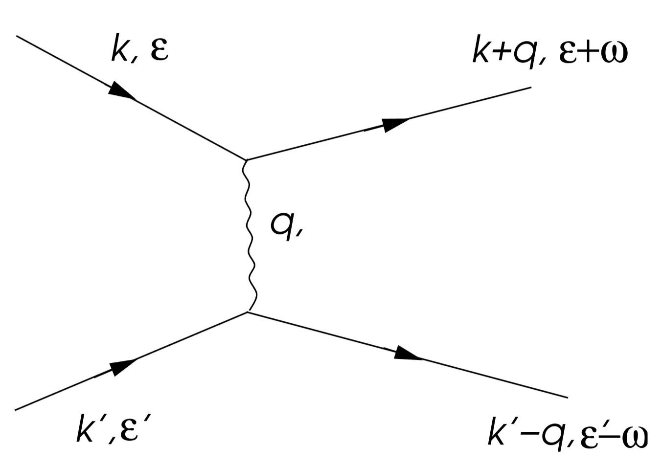
between the electrons is replaced in a metal by an effective interaction (with $q = | q |$ )

\begin{aligned} V_{ren} (q, ω) & = \frac{4 π e^{2}}{q^{2} ε (q, ω)} \\ = \frac{4 π e^{2}}{k_{T F}^{2} + q^{2}} (\frac{ω^{2}}{ω^{2} - ω_{q}^{2}}) . \end{aligned}

This interaction corresponds to the matrix element for a scattering process of two electrons with momentum exchange $q$ and energy exchange $ω$ . The phonon frequency $ω_{q}$ is always less than the Debye frequency $ω_{D}$ . Hence the effect of the phonons is almost irrelevant for energy exchanges $ω$ that are much larger than $ω_{D}$ . The time scale for such energies would be too short for the slow ions to move and influence the interaction. Interestingly, the repulsive bare Coulomb potential is renormalised to an interaction with an attractive channel for $ω < ω_{D}$ because of overcompensation by the ions. This aspect of the electron-phonon interaction is most important for superconductivity.

Attachments/Script 36.webp|700

3.4 Appendix: Linear Response Theory

Much information about a macroscopic system can be gained through the observation of its response to a small external perturbation. If the perturbation is sufficiently small we can consider the response of the system in lowest order, linear in the perturbing field. This is the approach pursued by the linear response theory.
If we knew all stationary states of a macroscopic quantum system with many degrees of freedom we could calculate essentially any desired quantity. However, the full information of such system is hard to store and is also unnecessary in view of our real experimental interests. The linear response functions are an efficient way to provide in a condensed form some of the most important and relevant information accessible in an experiment. The linear response function is one element of quantum field theory of solid-state physics. We will introduce it here on an elementary level.

3.4.1 Linear Response Function

Previously, we analysed the influence of an external potential on the distribution of electrons. The position- and time-dependent potential $V (r, t)$ induces the density modulation $δ n (r, t)$ which would be measured as a response to the potential. In real space and time the connection between the two is given by the linear relation,

\begin{array}{r} δ n (r, t) = \int d^{3} r^{'} \int d t^{'} χ (r - r^{'}, t - t^{'}) V (r^{'}, t^{'}) \end{array}

where we assume that the system is homogeneous and isotropic. The response function $χ (r - r^{'}, t - t^{'})$ describes how the potential at a position $r^{'}$ and time $t^{'}$ influences the behaviour of the system at the position $r$ and at a later time $t$ (causality). Causality actually requires that $χ (r, t) = 0$ for $t < 0$ . The response functions are non-local in space and time. The convolution can be converted into a simple product by going to momentum-frequency space,

\begin{array}{r} δ n (q, ω) = χ (q, ω) V (q, ω) \end{array}

where the Fourier transformation is performed as follows,

\begin{array}{r} f (r, t) = \frac{1}{Ω} \sum_{q} \int_{- \infty}^{+ \infty} \frac{d ω}{2 π} f (q, ω) e^{- i (ω t - q \cdot r)} . \end{array}

We now determine the response function for a general external field and response quantity.

Kubo formula - retarded Green's function

We consider a quantum system described by the Hamiltonian $H_{0}$ and analyze its response to an external field $ϕ (r, t)$ which couples to the field operator $\hat{A} (r)$ ,

\begin{array}{r} H = H_{0} + H^{'} (t) = H_{0} + \int d^{3} r \hat{A} (r) ϕ (r, t) e^{η t} \end{array}

where $η = 0_{+}$ is a small positive parameter allowing to switch the perturbation adiabatically on, that is, at time $t \to - \infty$ there is no perturbation. The behaviour of the system can be determined by the density matrix $\hat{ρ} (t)$ . Knowing $\hat{ρ}$ we can calculate interesting mean values of operators, $⟨ \hat{B} (t) ⟩ = tr (\hat{ρ} (t) \hat{B})$ . A way to find the density matrix goes via the equation of motion,

\begin{array}{r} i ℏ \frac{\partial \hat{ρ}}{\partial t} = - [\hat{ρ}, H] = - [\hat{ρ}, H_{0} + H^{'}] . \end{array}

We proceed using the concept of time-dependent perturbation theory, $\hat{ρ} = {\hat{ρ}}_{0} + δ \hat{ρ} (t)$ , with

\begin{array}{r} {\hat{ρ}}_{0} = \frac{1}{Z} e^{- β H_{0}} with Z = tr e^{- β H_{0}} \end{array}

as the partition function and insert this form into the equation of motion, which we then truncate at linear order in $H^{'}$ ,

\begin{array}{r} i ℏ \frac{\partial}{\partial t} δ \hat{ρ} = - [δ \hat{ρ}, H_{0}] - [{\hat{ρ}}_{0}, H^{'}] + \dots . \end{array}

We turn to the interaction representation (time-dependent perturbation theory),

\begin{aligned} δ \hat{ρ} (t) & = e^{- i H_{0} t / ℏ} \hat{y} (t) e^{i H_{0} t / ℏ} \\ ⟹ i ℏ \frac{\partial}{\partial t} δ \hat{ρ} & = - [δ \hat{ρ}, H_{0}] + e^{- i H_{0} t / ℏ} {i ℏ \frac{\partial \hat{y} (t)}{\partial t}} e^{i H_{0} t / ℏ} . \end{aligned}

Comparing the preceding equations for the density matrix and using the definition of the Hamiltonian we arrive at the equation for $\hat{y}$ ,

\begin{array}{r} i ℏ \frac{\partial \hat{y} (t)}{\partial t} = - [{\hat{ρ}}_{0}, H_{i n t}^{'} (t)] with H_{i n t}^{'} (t) = e^{i H_{0} t / ℏ} H^{'} e^{- i H_{0} t / ℏ} \end{array}

which is formally solved by

\begin{array}{r} \hat{y} (t) = \frac{i}{ℏ} \int_{- \infty}^{t} d t^{'} [{\hat{ρ}}_{0}, H_{i n t}^{'} (t^{'})] . \end{array}

We now look at the mean value of the observable $\hat{B} (r)$ . For simplicity we assume that the expectation value of $\hat{B}$ vanishes, if there is no perturbation, that is $⟨ \hat{B} ⟩_{0} = tr {{\hat{ρ}}_{0} \hat{B}} = 0$ . We determine

\begin{aligned} ⟨ \hat{B} (r) ⟩ (t) & = tr {δ \hat{ρ} (r, t) \hat{B} (r)} \\ = tr {\frac{i}{ℏ} e^{- i H_{0} t / ℏ} \int_{- \infty}^{t} d t^{'} [{\hat{ρ}}_{0}, H_{i n t}^{'} (t^{'})] e^{i H_{0} t / ℏ} \hat{B} (r)} . \end{aligned}

By means of cyclic permutation of the operators in ${\dots}$ , which does not affect the trace, we arrive at the form

\begin{aligned} ⟨ \hat{B} (r) ⟩ (t) & = - \frac{i}{ℏ} \int_{- \infty}^{t} d t^{'} \int d^{3} r^{'} tr {{\hat{ρ}}_{0} [{\hat{B}}_{i n t} (r, t), {\hat{A}}_{i n t} (r^{'}, t^{'})]} ϕ (r^{'}, t^{'}) e^{η t^{'}} \\ = \int d t^{'} \int d^{3} r^{'} χ_{B A} (r - r^{'}, t - t^{'}) ϕ (r^{'}, t^{'}) \end{aligned}

which defines the response function $χ_{B A}$ . Notably, it is entirely determined by the properties of the unperturbed system.

Kubo-Formula - Recipe for the linear response function: We arrive at the following recipe to obtain a general linear response function: We denote the Hamiltonian of the (unperturbed) system as $H_{0}$ . Then the linear response function of the pair of field operators $\hat{A} (r), \hat{B} (r)$ (they are often in practice conjugate operators, $\hat{A} = {\hat{B}}^{†}$ ) is given by

\begin{array}{r} χ_{B A} (r - r^{'}, t - t^{'}) = - \frac{i}{ℏ} Θ (t - t^{'}) {⟨ [{\hat{B}}_{H} (r, t), {\hat{A}}_{H} (r^{'}, t^{'})] ⟩}_{H_{0}} \end{array}

where $⟨ \dots ⟩_{H_{0}}$ is the thermal mean value with respect to the Hamiltonian $H_{0}$ ,

\begin{array}{r} ⟨ \hat{C} ⟩_{H_{0}} = \frac{tr {\hat{C} e^{- β H_{0}}}}{tr {e^{- β H_{0}}}} = \frac{tr {\hat{C} e^{- β H_{0}}}}{Z}, \end{array}

${\hat{A}}_{H} (t) = e^{i H_{0} t / ℏ} \hat{A} e^{- i H_{0} t / ℏ}$ is the Heisenberg representation of the operator $\hat{A}$ (analogous for $\hat{B}$ ). Note that the temporal step function $Θ (t - t^{'})$ ensures the causality, that is there is no response for the system before there is a perturbation. This form is often called Kubo formula or retarded Green's function.

3.4.2 Information in the Response Function

The information stored in the response function can be most easily visualised by assuming that we know the complete set of stationary states of the system Hamiltonian $H_{0} : H_{0} | n ⟩ = ϵ_{n} | n ⟩$ . For simplicity we will from now on assume that $\hat{A} = {\hat{B}}^{†}$ which is the case in many practical examples, and will simplify our notation. We can then rewrite the response function $χ$ as

\begin{aligned} χ (r - r^{'}, t - t^{'}) & = - \frac{i}{ℏ} Θ (t - t^{'}) \sum_{n} \frac{e^{- β ϵ_{n}}}{Z} {⟨ n | e^{i H_{0} t / ℏ} \hat{B} (r) e^{- i H_{0} t / ℏ} e^{i H_{0} t^{'} / ℏ} \hat{B} {(r^{'})}^{†} e^{- i H_{0} t^{'} / ℏ} | n ⟩ \\ - ⟨ n | e^{i H_{0} t^{'} / ℏ} \hat{B} {(r^{'})}^{†} e^{- i H_{0} t^{'} / ℏ} e^{i H_{0} t / ℏ} \hat{B} (r) e^{- i H_{0} t / ℏ} | n ⟩} \\ = - \frac{i}{ℏ} Θ (t - t^{'}) \sum_{n, n^{'}} \frac{e^{- β ϵ_{n}}}{Z} {⟨ n | \hat{B} (r) | n^{'} ⟩ ⟨ n^{'} | \hat{B} {(r^{'})}^{†} | n ⟩ e^{i (ϵ_{n} - ϵ_{n^{'}}) (t - t^{'}) / ℏ} \\ - ⟨ n | \hat{B} {(r^{'})}^{†} | n^{'} ⟩ ⟨ n^{'} | \hat{B} (r) | n ⟩ e^{i (ϵ_{n^{'}} - ϵ_{n}) (t - t^{'}) / ℏ}}, \end{aligned}

where we inserted $1 = \sum_{n^{'}} | n^{'} ⟩ ⟨ n^{'} |$ . It is convenient to work in $q$ - and $ω$ -space, reached via Fourier transformation,

\begin{aligned} χ (q, ω) & = \int d^{3} \tilde{r} \int_{- \infty}^{+ \infty} d \tilde{t} χ (\tilde{r}, \tilde{t}) e^{i ω \tilde{t} - i q \cdot \tilde{r}} \\ = - \frac{i}{ℏ Ω} \sum_{n, n^{'}} \frac{e^{- β ϵ_{n}}}{Z} {| ⟨ n | {\hat{B}}_{q} | n^{'} ⟩ |}^{2} \int_{0}^{\infty} d \tilde{t} {e^{i (ϵ_{n} - ϵ_{n^{'}} + ℏ ω) \tilde{t} / ℏ} - e^{i (ϵ_{n^{'}} - ϵ_{n} + ℏ ω) \tilde{t} / ℏ}} e^{- η \tilde{t}} \end{aligned}

where we introduce

\begin{array}{r} {\hat{B}}_{q} = \int d^{3} \tilde{r} \hat{B} (\tilde{r}) e^{- i q \cdot \tilde{r}} and {\hat{B}}_{q}^{†} = \int d^{3} \tilde{r} \hat{B} (\tilde{r})^{†} e^{i q \cdot \tilde{r}} . \end{array}

After the integration over time we obtain

\begin{aligned} χ (q, ω) & = \frac{1}{Ω} \sum_{n, n^{'}} \frac{e^{- β ϵ_{n}}}{Z} {| ⟨ n | {\hat{B}}_{q} | n^{'} ⟩ |}^{2} {\frac{1}{ℏ ω - ϵ_{n^{'}} + ϵ_{n} + i ℏ η} - \frac{1}{ℏ ω - ϵ_{n} + ϵ_{n^{'}} + i ℏ η}} \\ = \int_{0}^{\infty} d ω^{'} S (q, ω^{'}) {\frac{1}{ω - ω^{'} + i η} - \frac{1}{ω + ω^{'} + i η}} . \end{aligned}

In the last line we write the response function in a spectral form with $S (q, ω)$ as the spectral function,

\begin{array}{r} S (q, ω) = \frac{1}{Ω} \sum_{n, n^{'}} \frac{e^{- β ϵ_{n}}}{Z} {| ⟨ n | {\hat{B}}_{q} | n^{'} ⟩ |}^{2} δ (ℏ ω - ϵ_{n^{'}} + ϵ_{n}) . \end{array}

We call $S (q, ω)$ also dynamical structure factor which comprises information about the excitation spectrum associated with $\hat{B}$ . It represents a correlation function,

\begin{array}{r} S (r - r^{'}, t - t^{'}) = \frac{1}{ℏ} {⟨ {\hat{B}}_{H} (r, t) {\hat{B}}_{H} {(r^{'}, t^{'})}^{†} ⟩}_{H_{0}}, \end{array}

and contains the spectrum of the excitations which can be coupled to by the external perturbation.

Lindhard function

We show now how the Lindhard function is derived, where we restrict to independent electrons. Thus, we choose, $\hat{B} (r) = \sum_{s} {\hat{Ψ}}_{s} (r)^{†} {\hat{Ψ}}_{s} (r)$ which leads to

\begin{array}{r} {\hat{B}}_{q} = {\hat{ρ}}_{q} = \sum_{k, s} {\hat{c}}_{k s}^{†} {\hat{c}}_{k + q, s} = \sum_{k, s} {\hat{ρ}}_{k, q, s} . \end{array}

Now consider the matrix elements in

\begin{array}{r} \sum_{n, n^{'}} \frac{e^{- β ϵ_{n}}}{Z} ⟨ n | {\hat{c}}_{k s}^{†} {\hat{c}}_{k + q, s} | n^{'} ⟩ ⟨ n^{'} | {\hat{c}}_{k^{'} + q, s}^{†} {\hat{c}}_{k^{'} s} | n ⟩ = n_{0 k} (1 - n_{0 k + q}) δ_{k, k^{'}} \end{array}

for which

\begin{array}{r} ϵ_{n^{'}} = ϵ_{n} - ϵ_{k} + ϵ_{k + q} \Rightarrow ϵ_{n^{'}} - ϵ_{n} = ϵ_{k + q} - ϵ_{k} . \end{array}

The matrix element probes probability of whether the electron state with momentum $k$ is occupied, by $n_{k}$ , and the state $k + q$ , by $1 - n_{k + q}$ , is empty. Thus we obtain,

\begin{array}{r} χ (q, ω) = \frac{1}{Ω} \sum_{k} n_{0 k} (1 - n_{0 k + q}) {\frac{1}{ℏ ω - ϵ_{k + q} + ϵ_{k} + i ℏ η} - \frac{1}{ℏ ω + ϵ_{k + q} - ϵ_{k} + i ℏ η}} . \end{array}

The second term can be rewritten by substitution $k \to k - q$ and in a next step switch the sign of $q$ which leaves the result invariant, as our system has inversion symmetry. This leads then to

\begin{aligned} χ (q, ω) & = \frac{1}{Ω} \sum_{k} \frac{n_{0 k} (1 - n_{0 k + q}) - n_{0 k + q} (1 - n_{0 k})}{ℏ ω - ϵ_{k + q} + ϵ_{k} + i ℏ η} \\ = \frac{1}{Ω} \sum_{k} \frac{n_{0 k + q} - n_{0 k}}{ϵ_{k + q} - ϵ_{k} - ℏ ω - i ℏ η}, \end{aligned}

which is consistent with the Lindhard function defined previously. The Kubo formalism can be used to derive intensive response functions like the Lindhard function when appropriate normalization by volume is included.

3.4.3 Analytical Properties

The spectral representation of the linear response function shows that $χ_{B A} (q, ω)$ has poles only in the lower half of the complex $ω$ -plane. This property reflects causality ( $χ (r, t) = 0$ for $t < 0$ ). We separate now $χ = χ^{'} + i χ^{″}$ in real and imaginary part and use the relation

\begin{array}{r} lim_{η \to 0_{+}} \frac{1}{x + i η} = P \frac{1}{x} - i π δ (x) . \end{array}

with $P$ denoting the principal part. This relation leads to

\begin{aligned} χ^{'} (q, ω) & = \int_{0}^{\infty} d ω^{'} S (q, ω^{'}) {P \frac{1}{ω - ω^{'}} - P \frac{1}{ω + ω^{'}}}, \\ χ^{''} (q, ω) & = - π {S (q, ω) - S (q, - ω)} . \end{aligned}

Therefore the imaginary part of $χ$ corresponds to the excitation spectrum of the system. Finally, it has to be noted that $χ (q, ω)$ follows the Kramers-Kronig relations:

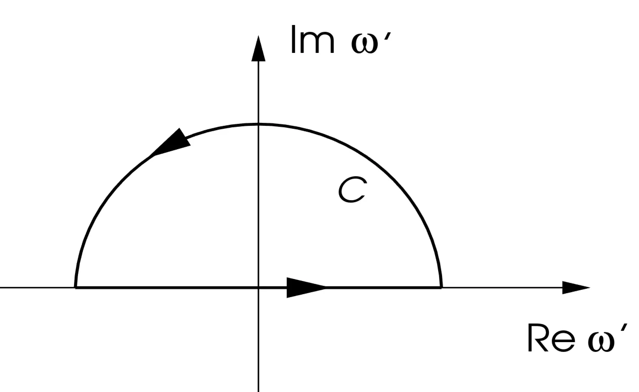
\begin{aligned} χ^{'} (q, ω) & = - \frac{1}{π} \int_{- \infty}^{+ \infty} d ω^{'} P \frac{χ^{''} (q, ω^{'})}{ω - ω^{'}} \\ χ^{''} (q, ω) & = \frac{1}{π} \int_{- \infty}^{+ \infty} d ω^{'} P \frac{χ^{'} (q, ω^{'})}{ω - ω^{'}} . \end{aligned}

Note to the Kramers-Kronig relation: This relation results from the analytic structure of $χ$ . Consider a contour in the upper half-plane of $ω^{'}$ where $χ (q, ω^{'})$ has no poles due to causality.

\begin{aligned} \oint_{C} d ω^{'} \frac{χ (q, ω^{'})}{ω^{'} - ω - i η^{'}} & = 0 \\ ⟹ \int_{- \infty}^{+ \infty} d ω^{'} χ (q, ω^{'}) P \frac{1}{ω^{'} - ω} + i π χ (q, ω) & = 0. \end{aligned}

Separating this equation into real and imaginary part yields the Kramers-Kronig relation.

Attachments/Script 37.webp|700

3.4.4 Fluctuation-Dissipation Theorem

First we consider the aspect of dissipation incorporated in the response function. For this purpose we ignore for simplicity the spatial dependence and consider a perturbative part of the Hamiltonian which only depends on time.

\begin{aligned} H^{'} & = \int d^{3} r \hat{B} (r) ϕ (r, t) \\ ⟹ ⟨ \hat{B} (r) ⟩ (t) & = \int_{0}^{\infty} d t^{'} \int d^{3} r^{'} χ (r - r^{'}, t - t^{'}) ϕ (r, t^{'}) \end{aligned}

with $\hat{B} = {\hat{B}}^{†}$ . We assume now a monochromatic external field,

\begin{aligned} ϕ (r, t) & = \frac{1}{2} (ϕ_{0} (r) e^{- i ω t} + ϕ_{0} (r)^{*} e^{i ω t}) \\ ⟹ ⟨ \hat{B} (r) ⟩ (t) & = \int_{0}^{\infty} d t^{'} \int d^{3} r^{'} χ (r - r^{'}, t - t^{'}) \frac{1}{2} (ϕ_{0} (r^{'}) e^{- i ω t^{'}} + ϕ_{0} {(r^{'})}^{*} e^{i ω t^{'}}) \\ = \frac{1}{2} \int d^{3} r^{'} {χ {(r - r^{'}, ω)}^{*} ϕ_{0} (r^{'}) e^{- i ω t} + χ (r - r^{'}, ω) ϕ_{0} (r^{'})^{*} e^{i ω t}} . \end{aligned}

The energy dissipation rate is determined by

\begin{aligned} \frac{d E}{d t} & = ⟨ \frac{\partial}{\partial t} H ⟩ = \int d^{3} r ⟨ \hat{B} (r) ⟩ (t) \frac{\partial ϕ (r, t)}{\partial t} \\ = \frac{1}{2} \int d^{3} r d^{3} r^{'} \frac{\partial ϕ (r, t)}{\partial t} {χ {(r - r^{'}, ω)}^{*} ϕ_{0} (r^{'}) e^{- i ω t} + χ (r - r^{'}, ω) ϕ_{0} (r^{'})^{*} e^{i ω t}} \\ = \frac{1}{2} \int d^{3} r d^{3} r^{'} i ω {ϕ_{0} (r) e^{- i ω t} + ϕ_{0} (r)^{*} e^{i ω t}} {χ {(r - r^{'}, ω)}^{*} ϕ_{0} (r^{'}) e^{- i ω t} + χ (r - r^{'}, ω) ϕ_{0} (r^{'})^{*} e^{i ω t}} \\ ⟹ \frac{\overset{―}{d E}}{d t} & = \frac{ω}{2} \iint d^{3} r d^{3} r^{'} ϕ_{0} (r)^{*} χ^{''} (r - r^{'}, ω) ϕ_{0} (r^{'}) = \sum_{q} \frac{ω}{2} χ^{''} (q, ω) | ϕ (q, ω) |^{2} < 0 \end{aligned}

where for the time averaged rate we drop oscillating terms with the time dependence $e^{\pm i 2 ω t} .$
The result before used the following: The time-derivative of the Hamiltonian is given by

\begin{array}{r} \frac{d H}{d t} = \frac{\partial H}{\partial t} + \frac{i}{ℏ} [H, H] = \frac{\partial H}{\partial t} \end{array}

for a quantum mechanical problem. The analogous relation is obtained for classical systems.

The imaginary part of the dynamical susceptibility describes the dissipation of the system and gives information about the spectrum and the density of excitations for given $q$ and $ω$ . From the definition of the dynamical structure factor it follows that

\begin{array}{r} S (q, - ω) = e^{- β ℏ ω} S (q, ω) \end{array}

because

\begin{aligned} S (q, - ω) & = \frac{1}{Ω} \sum_{n, n^{'}} \frac{e^{- β ϵ_{n}}}{Z} {| ⟨ n | {\hat{B}}_{q} | n^{'} ⟩ |}^{2} δ (- ℏ ω - ϵ_{n^{'}} + ϵ_{n}) \\ = \frac{1}{Ω} \sum_{n, n^{'}} \frac{e^{- β ϵ_{n^{'}} - β ℏ ω}}{Z} | ⟨ n^{'} | {\hat{B}}_{- q} | n ⟩ |^{2} δ (ℏ ω - ϵ_{n} + ϵ_{n^{'}}) = e^{- β ℏ ω} S (q, ω) . \end{aligned}

This is a statement of detailed balance. The transition matrix element between two states is the same whether the energy is absorbed or emitted. For emitting, however, the thermal occupation of the initial state has to be taken into account.
Using the relation $S (q, - ω) = e^{- β ℏ ω} S (q, ω)$ we can derive the following relation

\begin{array}{r} χ^{''} (q, ω) = - π [S (q, ω) - S (q, - ω)] = - π [1 - e^{- β ℏ ω}] S (q, ω) \end{array}

which is known as the fluctuation-dissipation theorem. Let us consider here some consequences and find the relation to our earlier simplified formulations.

\begin{aligned} \int_{- \infty}^{+ \infty} d ω S (q, ω) & = \int_{- \infty}^{+ \infty} d ω \frac{1}{Ω} \sum_{n, n^{'}} \frac{e^{- β ϵ_{n}}}{Z} {| ⟨ n | {\hat{B}}_{q} | n^{'} ⟩ |}^{2} δ (ℏ ω - ϵ_{n^{'}} + ϵ_{n}) \\ = \frac{1}{ℏ Ω} \sum_{n, n^{'}} \frac{e^{- β ϵ_{n}}}{Z} ⟨ n | {\hat{B}}_{q} | n^{'} ⟩ ⟨ n^{'} | {\hat{B}}_{q}^{†} | n ⟩ \\ = \frac{1}{ℏ} ⟨ {\hat{B}}_{q} (0) {\hat{B}}_{q}^{†} (0) ⟩ = - \frac{1}{π} \int_{- \infty}^{+ \infty} d ω \frac{χ^{''} (q, ω)}{1 - e^{- β ℏ ω}} \end{aligned}

This corresponds to the equal-time correlation function (assuming $⟨ \hat{B} ⟩ = 0$ ).

Now we turn to the classical case of the fluctuation-dissipation theorem and consider the limit $k_{B} T ≫ ℏ ω$ . Then we may approximate this equation by

\begin{array}{r} ⟨ | {\hat{B}}_{q} |^{2} ⟩ \approx - \frac{k_{B} T}{π} \int_{- \infty}^{+ \infty} d ω \frac{χ^{''} (q, ω)}{ω} = - k_{B} T χ^{'} (q, 0) = - k_{B} T χ (q, 0) . \end{array}

This is valid, if $χ^{''} (q, ω)$ essentially vanishes for frequencies comparable and larger than the temperature.
Static response function: We consider a system with

\begin{aligned} H & = H_{0} + H^{'} = H_{0} + \int d^{3} r h (r) \hat{B} (r) \\ = H_{0} + \frac{1}{V} \sum_{q} h_{- q} {\hat{B}}_{q} = H_{0} + \sum_{q} H_{- q} {\hat{B}}_{q} \end{aligned}

where we assume for the following ${\hat{B}}_{- q} = {\hat{B}}_{q}^{†}$ . The mean value

\begin{array}{r} ⟨ {\hat{B}}_{q} ⟩ = \frac{\partial F}{\partial H_{- q}} = - \frac{\partial}{\partial H_{- q}} k_{B} T \ln Z = tr (\hat{ρ} {\hat{B}}_{q}) \end{array}

with $\hat{ρ} = \exp [β (F - H)]$ and $⟨ {\hat{B}}_{q} ⟩ = 0$ for $H_{q} = 0$ . The static response function is obtain from

\begin{aligned} χ (q) & = {\frac{\partial ⟨ {\hat{B}}_{q} ⟩}{\partial H_{q}} |}_{H_{q} = 0} = {tr {{\hat{B}}_{q} \frac{\partial}{\partial H_{q}} e^{β (F - H)}} |}_{H_{q} = 0} \\ = {tr {{\hat{B}}_{q} β (⟨ {\hat{B}}_{- q} ⟩ - {\hat{B}}_{- q}) \hat{ρ}} |}_{H_{q} = 0} = - β ⟨ {\hat{B}}_{q} {\hat{B}}_{q}^{†} ⟩ \end{aligned}

which is the classical form of the fluctuation dissipation theorem for spatially modulated perturbative fields.
For a uniform field we find

\begin{array}{r} \int d^{3} r d^{3} r^{'} ⟨ \hat{B} (r, t = 0) {\hat{B}}^{†} (r^{'}, t = 0) ⟩ = ⟨ {\hat{B}}_{q = 0} {\hat{B}}_{q = 0}^{†} ⟩ = - k_{B} T χ (q = 0) = - k_{B} T χ \end{array}

that is the static uniform susceptibility is related to the integration of the equal-time correlation function as we had used previously several times. Note the minus sign results from the sign of coupling to the external field.