Jump back to chapter selection.

Table of Contents

1.1 Symmetries of Crystals
1.2 Bloch's Theorem and Bloch Functions
1.3 Nearly Free Electron Approximation
1.4 Tight-Binding Approximation
1.5 Symmetry Properties of the Band Structure
1.6 Band-Filling and Materials Properties
1.7 Dynamics of Band Electrons - Semiclassical Approach
1.8 Approximative Band Structure Calculations

1 Electrons in the Periodic Crystal

One defining characteristic of many solids is the regular arrangement of their atoms, forming a crystal. Electrons in such crystals experience a periodic potential, originating from the lattice of ions and the mean interaction with other electrons:

Attachments/Script.webp|700

The spectrum of these delocalised electronic states—solutions to the Schrödinger equation—forms energy bands separated by gaps of "forbidden" energies. Two limiting approaches help to understand this band formation:

Nearly-free electron approximation: A weak periodic potential breaks up the continuous spectrum into bands.
Tight-binding approximation: Independent atomic states overlap as atoms form a lattice, creating delocalised bands from discrete atomic energy levels.

1.1 Symmetries of Crystals

1.1.1 Space Groups of Crystals

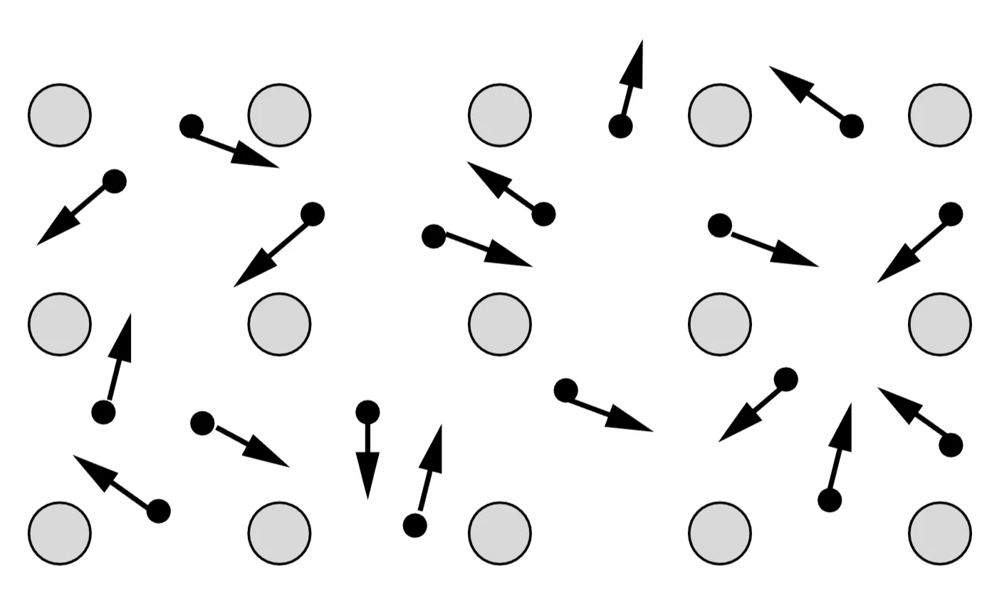
Most solids are built from a repeating lattice of atoms, with the smallest repeating unit known as the unit cell. The symmetries of a crystal are described by its space group $R$ , a collection of symmetry operations—translations, rotations, inversions, and combinations—that leave the crystal invariant. In three dimensions, there are 230 unique space groups.

We can visualise the crystal as a lattice of points, each representing either an atom or an entire unit cell. Translations within the space group are linear combinations of primitive lattice vectors ${a_{i}}$ :

R_{n} = n_{1} a_{1} + n_{2} a_{2} + n_{3} a_{3},

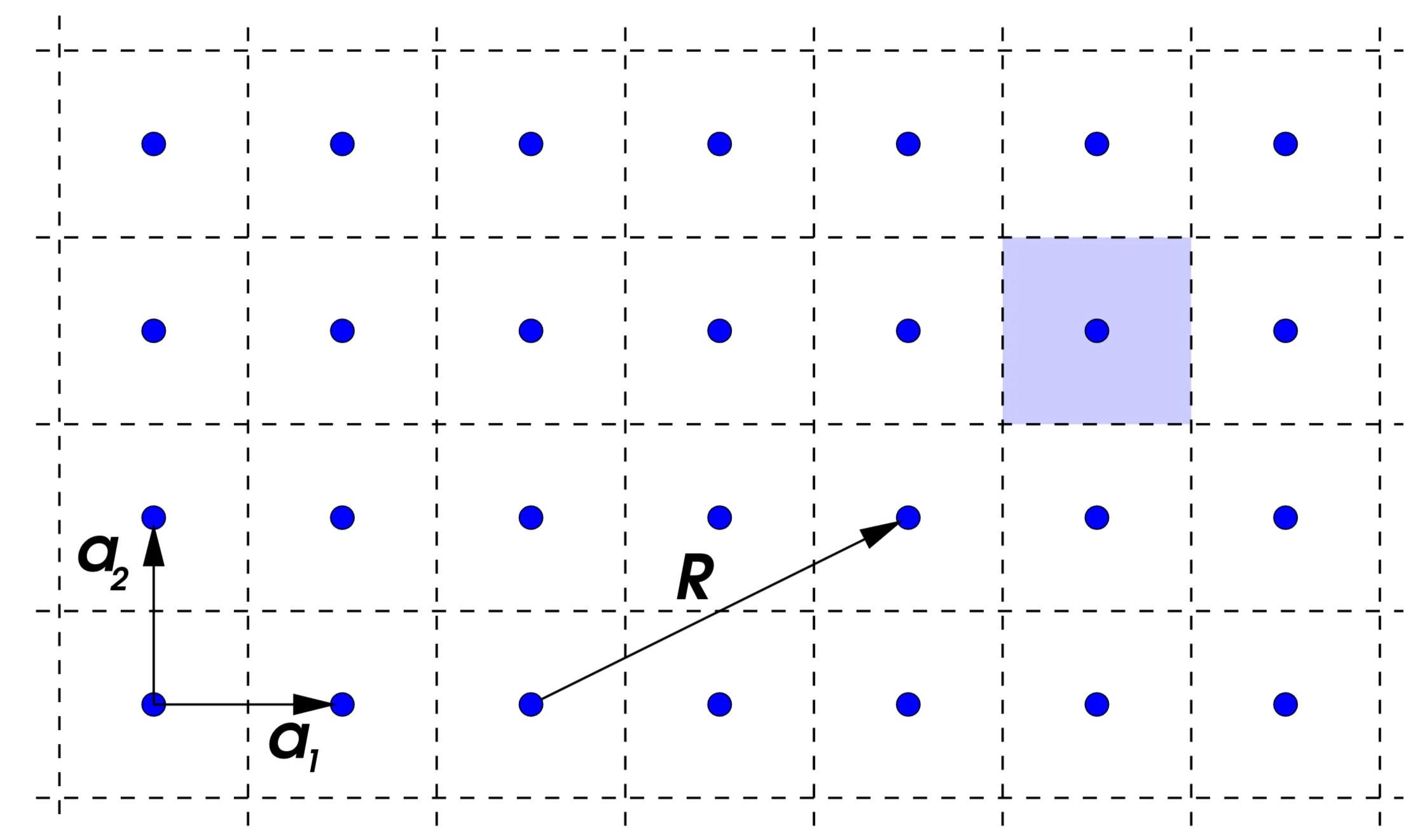
where $n = (n_{1}, n_{2}, n_{3})$ and $n_{i} \in Z$ . For example, in a 2D square lattice:

Attachments/Script 1.webp|700

Here, $a_{1}$ and $a_{2}$ are primitive lattice vectors, and $R = 2 a_{1} + a_{2}$ is a lattice vector. The shaded area is the Wigner-Seitz cell, a unit cell formed by bisecting lines connecting neighboring lattice points.

1.1.2 Symmetry Operations

Symmetry operations in the space group can be expressed in the Wigner notation:

r^{'} = g r + a = {g ∣ a} r,

where $g$ represents a rotation, reflection, or inversion with respect to specific points, axes, or planes. These operations generate the point group $P$ . Key symmetry operations include:

Operation	Notation
Basic translations	${E ∣ a}$
Rotations, reflections, inversions	${g ∣ 0}$
Screw axes, glide planes	${g ∣ a}$

Here, $E$ is the identity element of $P$ . A screw axis combines a rotation with a translation along the rotation axis, while a glide plane combines a reflection with a translation along the plane.

1.1.3 Group Properties

The space group $R$ satisfies the properties of a group:

Associativity: For any two elements ${g ∣ a}, {g^{'} ∣ a^{'}} \in R$ :
${g ∣ a} {g^{'} ∣ a^{'}} = {g g^{'} ∣ g a^{'} + a} .$
Identity Element: The identity is ${E ∣ 0}$ .
Inverse Element: For every ${g ∣ a} \in R$ , there exists an inverse:

\begin{aligned} {g ∣ a}^{- 1} & = {g^{- 1} ∣ - g^{- 1} a} \\ ⟹ {g ∣ a}^{- 1} {g ∣ a} & = {E ∣ 0} . \end{aligned}

In general, space group elements do not commute (non-Abelian group):

{g ∣ a} {g^{'} ∣ a^{'}} \neq {g^{'} ∣ a^{'}} {g ∣ a} .

However, the subgroup of translations ${{E ∣ a}} \subset R$ is always Abelian. Furthermore, the following relations hold generally:

\begin{aligned} {g ∣ a} {E ∣ a^{'}} {g ∣ a}^{- 1} & = {E ∣ g a^{'}}, \\ {g ∣ a}^{- 1} {E ∣ a^{'}} {g ∣ a} & = {E ∣ g^{- 1} a^{'}} . \end{aligned}

1.1.4 Reciprocal Lattice

The reciprocal lattice is a periodic lattice with its own translation symmetry, defined by a basic set of vectors ${b_{i}}$ . Any reciprocal lattice vector can be expressed as:

G_{m} = m_{1} b_{1} + m_{2} b_{2} + m_{3} b_{3},

where $m_{i}$ are integers. The relationship between the real lattice vectors ${a_{i}}$ and reciprocal lattice vectors ${b_{i}}$ is given by:

a_{i} \cdot b_{j} = 2 π δ_{i j}, i, j = 1, 2, 3,

with:

b_{i} = 2 π \frac{a_{j} \times a_{k}}{a_{i} \cdot (a_{j} \times a_{k})}, a_{i} = 2 π \frac{b_{j} \times b_{k}}{b_{i} \cdot (b_{j} \times b_{k})} .

For example, the reciprocal lattice of a simple cubic lattice is also simple cubic. However, a body-centered cubic (bcc) lattice corresponds to a face-centered cubic (fcc) reciprocal lattice, and vice versa.

A key property of real space lattice vectors $R_{n}$ and reciprocal lattice vectors $G_{m}$ is:

G_{m} \cdot R_{n} = 2 π (m_{1} n_{1} + m_{2} n_{2} + m_{3} n_{3}) = 2 π N,

where $N$ is an integer. This allows any function $f (r)$ periodic in the real lattice to be expanded as:

f (r) = \sum_{G} f_{G} e^{i G \cdot r},

with the periodic property $f (r + R) = f (r)$ . The expansion coefficients are:

f_{G} = \frac{1}{Ω_{UC}} \int_{UC} d^{3} r f (r) e^{- i G \cdot r},

where the integral runs over the unit cell of the periodic lattice with volume $Ω_{UC}$ . The first Brillouin zone is defined as the Wigner-Seitz cell of the reciprocal lattice.

1.2 Bloch's Theorem and Bloch Functions

Consider a Hamiltonian $H$ of electrons invariant under lattice translations ${E ∣ a}$ , introduced by a periodic potential. This implies that the translation operator ${\hat{T}}_{a}$ commutes with the Hamiltonian:

[{\hat{T}}_{a}, H] = 0.

The translation operator acts on the Hilbert space as:

{\hat{T}}_{a} | r ⟩ = | r + a ⟩, ⟨ r | {\hat{T}}_{a} = ⟨ r - a | .

Absorbing electron-electron interactions into an effective potential, the Hamiltonian reduces to:

H_{0} = \frac{{\hat{p}}^{2}}{2 m} + V (\hat{r}),

where $V (r) = \sum_{j} V_{ion} (r - R_{j})$ represents the periodic potential from ions and the mean field of other electrons. Since $V (r + a) = V (r)$ , $H_{0}$ commutes with ${\hat{T}}_{a}$ .

1.2.1 Bloch's Theorem

Bloch's theorem states that eigenvalues of ${\hat{T}}_{a}$ lie on the unit circle in the complex plane. This means:

{\hat{T}}_{a} ψ (r) = ψ (r - a) = λ_{a} ψ (r),

where $λ_{a} = e^{i φ_{a}}$ ensures bounded and delocalised wavefunctions. The eigenstates take the form:

ψ_{n, k} (r) = \frac{1}{\sqrt{Ω}} e^{i k \cdot r} u_{n, k} (r),

where $u_{n, k} (r)$ is periodic, and $n$ is the band index. The eigenfunctions satisfy:

H_{0} ψ_{n, k} (r) = ϵ_{n, k} ψ_{n, k} (r) .

1.2.2 Periodicity in Reciprocal Space

The eigenvalue $λ_{a} = e^{- i k \cdot a}$ implies periodicity in reciprocal space. For reciprocal lattice vectors $G$ :

ϵ_{n, k + G} = ϵ_{n, k}, ψ_{n, k + G} (r) = ψ_{n, k} (r) .

This reduces the discussion to the first Brillouin zone. Bloch's theorem simplifies the Schrödinger equation into the Bloch equation for $u_{k} (r)$ :

(\frac{(\hat{p} + ℏ k)^{2}}{2 m} + V (\hat{r})) u_{k} (r) = ϵ_{k} u_{k} (r),

where $\hat{p} e^{i k \cdot r} u_{k} (r) = e^{i k \cdot r} (\hat{p} + ℏ k) u_{k} (r)$ .

1.3 Nearly Free Electron Approximation

The nearly free electron approximation starts from the limit of free electrons, assuming the periodic potential $V (r)$ is weak and can be treated perturbatively. The periodic potential is expanded as:

V (r) = \sum_{G} V_{G} e^{i G \cdot r}, V_{G} = \frac{1}{Ω_{UC}} \int_{UC} d^{3} r V (r) e^{- i G \cdot r} .

Here, $V_{G}$ represents Fourier components of the potential, and $Ω_{UC}$ is the unit cell volume. The potential $V (r)$ is real and inversion-symmetric ( $V (r) = V (- r)$ ), leading to $V_{G} = V_{- G}$ . The uniform component $V_{0}$ is typically set to zero, as it only introduces a general energy shift.

The Bloch function, being periodic, is expressed similarly:

u_{k} (r) = \sum_{G} c_{G} e^{- i G \cdot r},

where $c_{G} = c_{G} (k)$ are $k$ -dependent coefficients. Inserting this into the Bloch equation along with the expansion for $V (r)$ , we obtain:

(\frac{ℏ^{2}}{2 m} (k - G)^{2} - ϵ_{k}) c_{G} + \sum_{G^{'}} V_{G^{'} - G} c_{G^{'}} = 0.

This represents an eigenvalue problem in infinite dimensions, where $c_{G} (k)$ are eigenvectors and $ϵ_{k}$ are eigenvalues, corresponding to the band energies. Without the potential $V (r)$ , the solutions form parabolic bands:

ϵ_{k} (G) = \frac{ℏ^{2}}{2 m} (k - G)^{2} .

This redundancy arises because every $G$ generates the same spectrum, satisfying $ϵ_{k + G} = ϵ_{k}$ . Restricting to the first Brillouin zone suffices to describe the complete energy spectrum. Within this zone, each $k$ corresponds to an infinite set of eigenvalues forming different bands.

1.3.1 Example: 1-Dimensional System

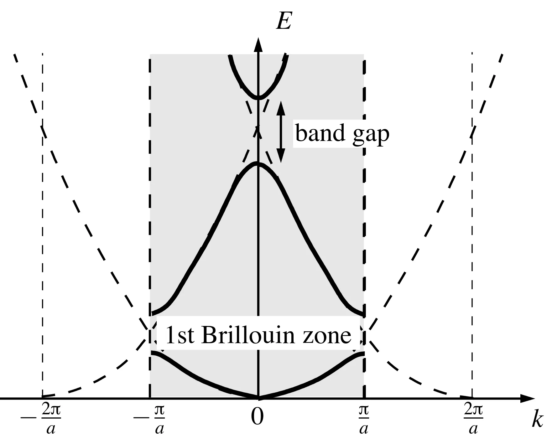
Consider a one-dimensional periodic lattice with lattice constant $a$ . The reciprocal lattice vector is $\tilde{G} = 2 π / a$ . Without a periodic potential, the bare spectrum is:

ϵ_{k} (G) = \frac{ℏ^{2}}{2 m} (k - G)^{2},

where $G = n \tilde{G}$ , corresponding to the dashed parabolas in the figure.

When a weak periodic potential is introduced with $| V_{G} | ≪ ℏ^{2} G^{2} / 2 m$ , the eigenvalue equation simplifies. Near the center of the Brillouin zone ( $k \approx 0$ ), the lowest energy band is non-degenerate, corresponding to:

ϵ_{k}^{(0)} = \frac{ℏ^{2} k^{2}}{2 m}, c_{0}^{(0)} = 1, c_{G}^{(0)} = 0 for G \neq 0.

The first-order correction to the Bloch function is:

c_{G}^{(1)} = \frac{- V_{G} c_{0}^{(0)}}{\frac{ℏ^{2}}{2 m} ((k - G)^{2} - k^{2})} \approx - \frac{λ_{G}}{1 - 2 k / G},

where $λ_{G} = V_{G} / (ℏ^{2} G^{2} / 2 m)$ is the small perturbation parameter.

The corrected energy eigenvalues are:

ϵ_{k} \approx ϵ_{k}^{(0)} - \sum_{G \neq 0} \frac{| V_{G} |^{2}}{\frac{ℏ^{2}}{2 m} [(k - G)^{2} - k^{2}]} \approx \frac{ℏ^{2} k^{2}}{2 m^{*}} + E_{0},

where:

E_{0} = - \sum_{G \neq 0} | λ_{G} |^{2} \frac{ℏ^{2} G^{2}}{2 m}, \frac{1}{m^{*}} = \frac{1}{m} (1 - 4 \sum_{G \neq 0} | λ_{G} |^{2}) .

This modifies the dispersion relation, yielding an effective mass $m^{*} > m$ , as shown in the figure:

Attachments/Script 2.webp|700

The $k \cdot p$ approximation describes this expansion near symmetry points. The next energy level at $k = 0$ results from two crossing parabolas centered at $G_{\pm} = \pm 2 π / a = \pm \tilde{G}$ . Restricting to these components, the eigenvalue problem simplifies to:

(\begin{array}{cc} \frac{ℏ^{2}}{2 m} (k - \tilde{G})^{2} - ϵ_{k} & V_{- 2 \tilde{G}} \\ V_{2 \tilde{G}} & \frac{ℏ^{2}}{2 m} (k + \tilde{G})^{2} - ϵ_{k} \end{array}) (\binom{c_{+ \tilde{G}}}{c_{- \tilde{G}}}) = 0.

The eigenvalues are:

ϵ_{k \pm} \approx \frac{ℏ^{2}}{2 m} {\tilde{G}}^{2} \pm | V_{2 \tilde{G}} | + \frac{ℏ^{2}}{2 m_{\pm}^{*}} k^{2},

with effective masses:

\frac{1}{m_{\pm}^{*}} \approx \frac{1}{m} (1 \pm \frac{1}{2 | λ_{2 \tilde{G}} |}) .

Here, $m_{+}^{*} > 0$ and $m_{-}^{*} < 0$ correspond to bands with opposite curvatures, separated by a band gap. For $V_{2 \tilde{G}} \to 0$ , the curvature diverges as $m_{\pm}^{*} \to 0$ . The wavefunctions at $k = 0$ are:

u_{k = 0} (x) = {\begin{cases} \sin (\tilde{G} x), & ϵ_{k = 0, +}, \\ \cos (\tilde{G} x), & ϵ_{k = 0, -} . \end{cases}

These states correspond to bonding and antibonding states under parity $x \to - x$ . Similar band gaps occur at the Brillouin zone boundary ( $k = \pm π / a$ ). The energy spectrum is periodic, satisfying $ϵ_{k + G} = ϵ_{k}$ and $ϵ_{- k} = ϵ_{+ k}$ due to parity and time-reversal symmetry.

1.3.2 Appendix: Nearly Free Electron Approximation - Rayleigh-Schrödinger Formulation

We treat here the nearly free electron approximation for the one-dimensional system within the Rayleigh-Schrödinger perturbation theory. For this purpose we introduce the Dirac notation and write the plane wave state for free electrons as $| k ⟩$ with

\begin{array}{r} H_{0} = \frac{{\hat{p}}^{2}}{2 m} H_{0} | k ⟩ = \frac{ℏ^{2} k^{2}}{2 m} | k ⟩ = ϵ_{k}^{(0)} | k ⟩ \end{array}

The periodic potential $\hat{V}$ has the property

\begin{aligned} \hat{V} | k ⟩ & = \sum_{k^{'}} | k^{'} ⟩ ⟨ k^{'} | \hat{V} | k ⟩ \\ = \sum_{G} | k + G ⟩ ⟨ k + G | \hat{V} | k ⟩ = \sum_{G} V_{G} | k + G ⟩ \end{aligned}

where we use that $⟨ k^{'} | \hat{V} | k ⟩$ is only non-vanishing, if $k - k^{'} = G$ a reciprocal lattice vector. We now approximate the eigenstates and eigenenergies. We notice that for given $k$ the relevant subspace of the Hilbert-space is ${| k + G ⟩}$ including all $G$ . Thus the Bloch states can be written as

\begin{array}{r} | ψ_{k} ⟩ = \sum_{G} c_{G} | k - G ⟩ . \end{array}

First we consider the situation around $k \approx 0$ for the lowest energy state. Within perturbation theory we obtain

\begin{aligned} | ψ_{k} ⟩ & \approx | k ⟩ - \sum_{G \neq 0} | k - G ⟩ \frac{⟨ k - G | \hat{V} | k ⟩}{ϵ_{k - G}^{(0)} - ϵ_{k}^{(0)}} \\ = | k ⟩ - \sum_{G \neq 0} \frac{V_{- G}}{ϵ_{k - G}^{(0)} - ϵ_{k}^{(0)}} | k - G ⟩ \end{aligned}

and the energy is given by

\begin{aligned} ϵ_{k} & \approx ϵ_{k}^{(0)} + ⟨ k | \hat{V} | k ⟩ - \sum_{G \neq 0} \frac{{| ⟨ k - G | \hat{V} | k ⟩ |}^{2}}{ϵ_{k - G}^{(0)} - ϵ_{k}^{(0)}} \\ = ϵ_{k}^{(0)} + V_{0} - \sum_{G \neq 0} \frac{{| V_{- G} |}^{2}}{ϵ_{k - G}^{(0)} - ϵ_{k}^{(0)}} . \end{aligned}

Note that the definitions of $V_{G}$ and $c_{G}$ are in line with those used in Section 1.3. For the potential,

\begin{aligned} V (x) & = ⟨ x | \hat{V} | x ⟩ = \sum_{k, k^{'}} ⟨ x ∣ k^{'} ⟩ \underset{V_{G} δ_{k^{'}, k + G}}{\underset{⏟}{⟨ k^{'} | \hat{V} | k ⟩}} ⟨ k ∣ x ⟩ \\ = \sum_{k, G} V_{G} ⟨ x ∣ k + G ⟩ ⟨ k ∣ x ⟩ = \sum_{G} V_{G} e^{i G x} \end{aligned}

where we use $⟨ x ∣ k ⟩ = \frac{1}{\sqrt{L}} e^{i k x}$ with $L$ the length of the system. Note that $\frac{1}{L} \sum_{k} 1 = 1$ . For the Bloch function we find,

\begin{aligned} ψ_{k} (x) & = ⟨ x ∣ ψ_{k} ⟩ = \sum_{G} c_{G} ⟨ x ∣ k - G ⟩ \\ = \frac{1}{\sqrt{L}} e^{i k x} \sum_{G} c_{G} e^{- i G x} = \frac{1}{\sqrt{L}} e^{i k x} u_{k} (x) . \end{aligned}

After the non-degenerate energy level we consider the case where two states are "nearly" degenerate. For example, $| k + \tilde{G} ⟩$ and $| k - \tilde{G} ⟩$ with $\tilde{G} = 2 π / a$ , with the energies $ϵ_{k + \tilde{G}}^{(0)}$ and $ϵ_{k - \tilde{G}}^{(0)}$ , respectively, which are identical at $k = 0$ . We treat this situation within the scheme of degenerate perturbation theory by restricting to the subspace of these two states, writing the state as $| ψ_{k} ⟩ = c_{+ \tilde{G}} | k + \tilde{G} ⟩ + c_{- \tilde{G}} | k - \tilde{G} ⟩$ . The Schrödinger equation is given by

\begin{array}{r} H | ψ_{k} ⟩ = E_{k} | ψ_{k} ⟩ ⟹ {\begin{cases} ⟨ k + \tilde{G} | H | ψ_{k} ⟩ = E_{k} c_{+ \tilde{G}} \\ ⟨ k - \tilde{G} | H | ψ_{k} ⟩ = E_{k} c_{- \tilde{G}} \end{cases} \end{array}

such that

\begin{array}{r} (\begin{array}{cc} ϵ_{k + \tilde{G}}^{(0)} - E_{k} & V_{2 \tilde{G}} \\ V_{- 2 \tilde{G}} & ϵ_{k - \tilde{G}}^{(0)} - E_{k} \end{array}) (\binom{c_{+ \tilde{G}}}{c_{- \tilde{G}}}) = 0 \end{array}

is an eigenvalue equation with

\begin{aligned} E_{k, \pm} & = \frac{1}{2} [ϵ_{k + \tilde{G}}^{(0)} + ϵ_{k - \tilde{G}}^{(0)} \pm \sqrt{{(ϵ_{k + \tilde{G}}^{(0)} - ϵ_{k - \tilde{G}}^{(0)})}^{2} + 4 {| V_{2 \tilde{G}} |}^{2}}] \\ \approx \frac{ℏ^{2} {\tilde{G}}^{2}}{2 m} \pm | V_{2 \tilde{G}} | + \frac{ℏ^{2} k^{2}}{2 m_{\pm}^{*}} \end{aligned}

with an effective mass $m_{\pm}^{*} .$ The eigenstate is given by

\begin{array}{r} c_{+ \tilde{G}}^{(\pm)} (k) = \frac{- V_{2 \tilde{G}}}{\sqrt{{(ϵ_{k + \tilde{G}}^{(0)} - E_{k, \pm})}^{2} + {| V_{2 \tilde{G}} |}^{2}}} \end{array}

and

\begin{array}{r} c_{- \tilde{G}}^{(\pm)} (k) = \frac{ϵ_{k + \tilde{G}}^{(0)} - E_{k, \pm}}{\sqrt{{(ϵ_{k + \tilde{G}}^{(0)} - E_{k, \pm})}^{2} + {| V_{2 \tilde{G}} |}^{2}}} . \end{array}

We find the following relations for the wave functions,

\begin{array}{r} (c_{+ \tilde{G}}^{(\pm)} (k), c_{- \tilde{G}}^{(\pm)} (k)) \to {\begin{cases} (\frac{1}{\sqrt{2}}, \pm \frac{1}{\sqrt{2}}) & k = 0 \\ (\frac{1 \pm 1}{2}, \frac{1 \mp 1}{2}), & k ≫ | λ_{2 \tilde{G}} | \tilde{G} \\ (\frac{1 \mp 1}{2}, \frac{1 \pm 1}{2}), & k ≪ - | λ_{2 \tilde{G}} | \tilde{G} \end{cases} \end{array}

This means that the two states are completely hybridised at the point of degeneracy $(k = 0)$ while if $k$ is shifted sufficiently far away from this point, the wave functions reduce to the original states $| k \pm \tilde{G} ⟩$ . Thus, the opening of the band gap at $k = 0$ is an effect of hybridisation. The analysis can be done equivalently for every degeneracy point in $k$ . In our one-dimensional system these are always points of degeneracy 2 unlike in higher dimensional lattices.

1.4 Tight-Binding Approximation

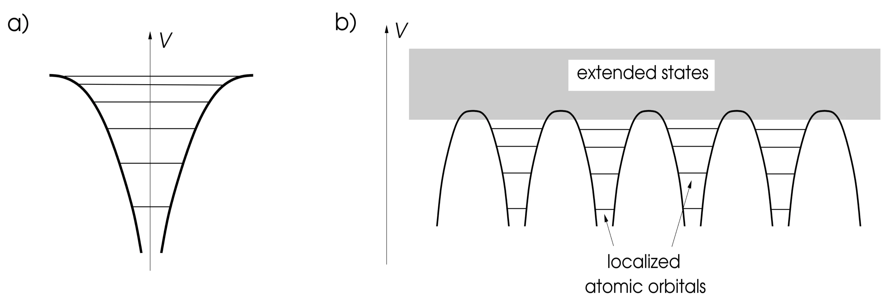
The tight-binding approximation starts from the atomic limit, considering a lattice of well-separated atoms where the overlap between the outermost electronic orbitals is small. In this scenario, electronic states are well-approximated by localised atomic orbitals $ϕ_{n} (r)$ . These orbitals are solutions to the atomic Hamiltonian:

H_{a} (R) ϕ_{n} (r - R) = ϵ_{n} ϕ_{n} (r - R),

where $H_{a} (R)$ is defined as:

H_{a} (R) = \frac{{\hat{p}}^{2}}{2 m} + V_{a} (r - R),

and $V_{a} (r)$ is the rotationally symmetric atomic potential. The potential landscape is depicted below, showing (a) the discrete spectrum of a single atomic Coulomb potential and (b) the periodic potential arising from a regular lattice:

Attachments/Script 3.webp|700

At low energies, electrons remain localised near atomic sites, but at higher energies, wavefunctions extend further and can delocalise to form itinerant states, leading to band formation.

The periodic single-particle Hamiltonian for the lattice is:

H = \frac{{\hat{p}}^{2}}{2 m} + \sum_{R_{j}} V_{a} (r - R_{j}) = H_{a} (R_{i}) + Δ V_{R_{i}} (r),

where $R_{i}$ is an arbitrary atomic position and:

Δ V_{R_{i}} (r) = \sum_{R_{j} \neq R_{i}} V_{a} (r - R_{j}) .

1.4.1 Linear Combination of Atomic Orbitals (LCAO)

Extended Bloch states can be approximated by a linear combination of atomic orbitals:

ψ_{\tilde{n} k} (r) = \frac{1}{\sqrt{N}} \sum_{R_{j}} e^{i k \cdot R_{j}} ϕ_{\tilde{n}} (r - R_{j}),

where $N$ is the number of atomic positions. This construction satisfies the Bloch condition:

ψ_{\tilde{n} k} (r - a) = e^{- i k \cdot a} ψ_{\tilde{n} k} (r),

for all lattice vectors $a$ .

The eigenstates of the Hamiltonian can be expressed as:

ψ_{k} (r) = \sum_{\tilde{n}} A_{\tilde{n}} ψ_{\tilde{n} k} (r),

which remains a Bloch wavefunction. This formulation allows deriving the electronic spectrum from:

H ψ_{k} (r) = ϵ_{k} ψ_{k} (r) .

By projecting onto the atomic orbitals, the problem reduces to the algebraic eigenvalue equation:

\sum_{{\tilde{n}}^{'}} [⟨ H ⟩_{\tilde{n} {\tilde{n}}^{'}} (k) - ϵ_{k} ⟨ 1 ⟩_{\tilde{n} {\tilde{n}}^{'}} (k)] A_{{\tilde{n}}^{'}} = 0,

with matrix elements:

⟨ 1 ⟩_{\tilde{n} {\tilde{n}}^{'}} (k) = \int d^{3} r ψ_{\tilde{n} k}^{*} (r) ψ_{{\tilde{n}}^{'} k} (r),

and:

⟨ H ⟩_{\tilde{n} {\tilde{n}}^{'}} (k) = \int d^{3} r ψ_{\tilde{n} k}^{*} (r) H ψ_{{\tilde{n}}^{'} k} (r) .

Using translational invariance, the matrix elements simplify to include terms involving nearest- or next-nearest-neighbor lattice sites.

1.4.2 Band Structure Calculation

The energy spectrum is obtained from the secular equation:

\det [⟨ H ⟩_{\tilde{n} {\tilde{n}}^{'}} (k) - ϵ_{k} ⟨ 1 ⟩_{\tilde{n} {\tilde{n}}^{'}} (k)] = 0.

The tight-binding approach is particularly effective for systems where atomic orbitals are tightly localised, such as 3d orbitals in transition metals (for example, Mn, Fe, Co) or transition metal oxides. For elements like alkali metals with delocalised s-orbitals, this approximation is less suitable. Explicit calculation of s and p orbitals skipped.

1.4.3 Wannier Functions

An alternative approach to the tight-binding approximation is through Wannier functions, which are defined as the Fourier transform of the Bloch wave functions:

\begin{aligned} ψ_{k} (r) & = \frac{1}{\sqrt{N}} \sum_{R} e^{i k \cdot R} w (r - R), \\ w (r - R) & = \frac{1}{\sqrt{N}} \sum_{k} e^{- i k \cdot R} ψ_{k} (r), \end{aligned}

where the Wannier function $w (r - R)$ is localised at the real-space lattice site $R$ . However, the Wannier function is not uniquely defined due to "gauge freedom," which allows multiplication of the Bloch function by an arbitrary phase factor:

ψ_{k} (r) \to e^{i χ (k)} ψ_{k} (r),

where $χ (k)$ is any real function. The degree of localisation of $w (r - R)$ around its center $R$ depends on the choice of $χ (k)$ .

For a non-degenerate band, similar to the atomic $s$ -orbital case, there is one Wannier function per site. These functions obey the orthogonality relation:

\int d^{3} r w^{*} (r - R^{'}) w (r - R) = δ_{R R^{'}} .

Considering a one-particle Hamiltonian $H = - \frac{ℏ^{2}}{2 m} \nabla^{2} + V (r)$ with a periodic potential $V (r)$ , the energy $ϵ_{k}$ can be expressed as:

ϵ_{k} = \int d^{3} r ψ_{k}^{*} (r) H ψ_{k} (r) .

Using the Fourier representation of the Bloch and Wannier functions:

ϵ_{k} = \sum_{R} e^{- i k \cdot R} \int d^{3} r w^{*} (r - R) H w (r),

where translational invariance is applied. Defining:

\begin{aligned} ϵ_{0} & = \int d^{3} r w^{*} (r) H w (r), \\ t (R) & = \int d^{3} r w^{*} (r - R) H w (r), \end{aligned}

the band energy becomes:

ϵ_{k} = ϵ_{0} + \sum_{R} t (R) e^{- i k \cdot R} .

This result mirrors the tight-binding band structure derived earlier via the LCAO approach.

For multiple bands (for example, $p$ -orbitals), we define:

ψ_{n k} (r) = \frac{1}{\sqrt{N}} \sum_{R, \tilde{n}} e^{i k \cdot R} c_{n \tilde{n}} (k) w_{\tilde{n}} (r - R),

where the matrix $c_{n \tilde{n}} (k)$ rotates the Wannier functions from the band basis to the atomic orbital basis. The coefficients satisfy:

\sum_{\tilde{n}} c_{n \tilde{n}} (k) c_{\tilde{n} n^{'}}^{*} (k) = δ_{n n^{'}} .

The band energy for multi-band systems can be expressed as:

ϵ_{n k} = \sum_{R} \sum_{\tilde{n}, {\tilde{n}}^{'}} c_{{\tilde{n}}^{'} n}^{*} (k) c_{n \tilde{n}} (k) e^{- i k \cdot R} t_{{\tilde{n}}^{'} \tilde{n}} (R),

where $t_{{\tilde{n}}^{'} \tilde{n}} (R)$ represents the hopping amplitudes. This approach works well for systems with well-localised orbitals.

1.4.4 Tight Binding Model in Second Quantisation Formulation

The tight-binding formulation of band electrons can also be implemented very easily in second quantisation language and provides a rather intuitive interpretation. For simplicity we restrict ourselves to the single-orbital case and define the following Fermionic operators,

\begin{array}{r} \begin{aligned} {\hat{c}}_{j, s}^{†} creates an electron of spin s on lattice site R_{j}, \\ {\hat{c}}_{j, s} annihilates an electron of spin s on lattice site R_{j}, \end{aligned} \end{array}

in the corresponding Wannier states. We introduce the following Hamiltonian,

\begin{array}{r} H = \sum_{j, s} ϵ_{0} {\hat{c}}_{j, s}^{†} {\hat{c}}_{j, s} + \sum_{i, j} t_{i j} {\hat{c}}_{i, s}^{†} {\hat{c}}_{j, s} \end{array}

with $t_{i j} = t_{j i}$ real. These coefficients $t_{i j}$ are called "hopping matrix elements", since ${\hat{c}}_{i, s}^{†} {\hat{c}}_{j, s}$ annihilates an electron on site $R_{j}$ and creates one on site $R_{i}$ , in this way an electron moves (hops) from $R_{j}$ to $R_{i}$ . Thus, this Hamiltonian represents the "kinetic energy" of the electron. Let us now diagonalise this Hamiltonian by following Fourier transformation, equivalent to the transformation between Bloch and Wannier functions,

\begin{array}{r} {\hat{c}}_{j, s}^{†} = \frac{1}{\sqrt{N}} \sum_{k} {\hat{a}}_{k s}^{†} e^{- i k \cdot R_{j}} and {\hat{c}}_{j, s} = \frac{1}{\sqrt{N}} \sum_{k} {\hat{a}}_{k s} e^{i k \cdot R_{j}} \end{array}

where ${\hat{a}}_{k s}^{†} ({\hat{a}}_{k s})$ creates (annihilates) an electron in the Bloch state with lattice momentum $k$ and spin $s$ . This leads to

\begin{aligned} H & = \sum_{k, k^{'}, s} {\frac{1}{N} \sum_{i} ϵ_{0} e^{i (k - k^{'}) \cdot R_{i}} + \frac{1}{N} \sum_{i, j} t_{i j} e^{i k \cdot R_{j} - i k^{'} \cdot R_{i}}} {\hat{a}}_{k^{'} s}^{†} {\hat{a}}_{k s} \\ = \sum_{k, s} ϵ_{k} {\hat{a}}_{k s}^{†} {\hat{a}}_{k s} \end{aligned}

where ${\hat{a}}_{k s}^{†} {\hat{a}}_{k s} = {\hat{n}}_{k s}$ constitutes the number operator for electrons. The band energy $ϵ_{k}$ is the same as obtained above from the tight-binding approach. The Hamiltonian formulation shown above will be used later for the Hubbard model where a real-space formulation is helpful.
The real-space formulation of the kinetic energy allows also for the introduction of disorder, nonperiodicity which can be most straightforwardly implemented by site dependent potentials $ϵ_{0} \to ϵ_{0 i}$ and to spatially (bond) dependent hopping matrix elements $t_{i j} = t (R_{i}, R_{j}) \neq t (R_{i} - R_{j})$ .

1.5 Symmetry Properties of the Band Structure

The symmetry properties of crystals are a helpful tool for the analysis of their band structure. They emerge from the symmetry group (space and point group) of the crystal lattice. Consider the action ${\hat{S}}_{{g ∣ a}}$ of an element ${g ∣ a}$ of the space group on a Bloch wave function $ψ_{k} (r)$

\begin{array}{r} {\hat{S}}_{{g ∣ a}} ψ_{k} (r) = ψ_{k} ({g ∣ a}^{- 1} r) = ψ_{k} (g^{- 1} r - g^{- 1} a) . \end{array}

Note that in Dirac notation we write for the Bloch state with lattice momentum $k$ as

\begin{array}{r} ψ_{k} (r) = ⟨ r ∣ ψ_{k} ⟩ \end{array}

The action of the operator ${\hat{S}}_{{g ∣ a}}$ on the state $| r ⟩$ is given by

\begin{array}{r} {\hat{S}}_{{g ∣ a}} | r ⟩ = | g r + a ⟩ and ⟨ r | {\hat{S}}_{{g ∣ a}} = ⟨ g^{- 1} r - g^{- 1} a |, \end{array}

such that

\begin{array}{r} ⟨ r | {\hat{S}}_{{g ∣ a}} | ψ_{k} ⟩ = ψ_{k} (g^{- 1} r - g^{- 1} a) . \end{array}

The same holds for pure translations. Note also that this definition has also implications on the sequential application of transformation operators such as

\begin{aligned} {\hat{S}}_{{g_{1} ∣ a_{1}}} {\hat{S}}_{{g_{2} ∣ a_{2}}} ψ_{k} (r) & = ⟨ r | {\hat{S}}_{{g_{1} ∣ a_{1}}} {\hat{S}}_{{g_{2} ∣ a_{2}}} | ψ_{k} ⟩ \\ = ⟨ {g_{1} ∣ a_{1}}^{- 1} r | {\hat{S}}_{{g_{2} ∣ a_{2}}} | ψ_{k} ⟩ \\ = ⟨ {g_{2} ∣ a_{2}}^{- 1} {g_{1} ∣ a_{1}}^{- 1} r ∣ ψ_{k} ⟩ \\ = ψ_{k} ({g_{2} ∣ a_{2}}^{- 1} {g_{1} ∣ a_{1}}^{- 1} r) \end{aligned}

Because ${g ∣ a}$ belongs to the space group of the crystal, we have $[{\hat{S}}_{{g ∣ a}}, H_{0}] = 0$ . Applying a pure translation ${\hat{T}}_{a^{'}} = {\hat{S}}_{{E ∣ a^{'}}}$ to this new wave function,

\begin{aligned} {\hat{T}}_{a^{'}} {\hat{S}}_{{g ∣ a}} ψ_{k} (r) & = {\hat{S}}_{{g ∣ a}} {\hat{T}}_{g^{- 1} a^{'}} ψ_{k} (r) = {\hat{S}}_{{g ∣ a}} e^{- i k \cdot (g^{- 1} a^{'})} ψ_{k} (r) \\ = {\hat{S}}_{{g ∣ a}} e^{- i (g k) \cdot a^{'}} ψ_{k} (r) \\ = e^{- i (g k) \cdot a^{'}} {\hat{S}}_{{g ∣ a}} ψ_{k} (r), \end{aligned}

the latter is found to be an eigenfunction of ${\hat{T}}_{a^{'}}$ with eigenvalue $e^{- i (g k) \cdot a^{'}}$ . Remember that, according to Bloch's theorem, we chose a basis ${ψ_{k}}$ diagonalising both ${\hat{T}}_{a}$ and $H_{0}$ . Thus, apart from a phase factor, the action of a symmetry transformation ${g ∣ a}$ on the wave function corresponds to a rotation from $k$ to $g k$ .

\begin{array}{r} {\hat{S}}_{{g ∣ a}} ψ_{k} (r) = λ_{{g ∣ a}} ψ_{g k} (r) \end{array}

with ${| λ_{{g ∣ a}} |}^{2} = 1$ , or

\begin{array}{r} {\hat{S}}_{{g ∣ a}} | k ⟩ = λ_{{g ∣ a}} | g k ⟩ . \end{array}

in Dirac notation. Here we used the symmetry behaviour of the wave function:

\begin{aligned} {\hat{S}}_{{g ∣ a}} ψ_{k} (r) & = \frac{1}{\sqrt{Ω}} {\hat{S}}_{{g ∣ a}} e^{i k \cdot r} \sum_{G} c_{G} (k) e^{i G \cdot r} = \frac{1}{\sqrt{Ω}} e^{i k \cdot (g^{- 1} r - g^{- 1} a)} \sum_{G} c_{G} (k) e^{i G \cdot (g^{- 1} r - g^{- 1} a)} \\ = \frac{1}{\sqrt{Ω}} e^{- i (g k) \cdot a} e^{i (g k) \cdot r} \sum_{G} c_{G} (k) e^{i (g G) \cdot r} = e^{- i (g k) \cdot a} \frac{1}{\sqrt{Ω}} e^{i (g k) \cdot r} \sum_{G} c_{g^{- 1} G} (k) e^{i G \cdot r} \\ = e^{- i (g k) \cdot a} \frac{1}{\sqrt{Ω}} e^{i (g k) \cdot r} \sum_{G} c_{G} (g k) e^{i G \cdot r} = λ_{{g ∣ a}} ψ_{g k} (r) \end{aligned}

where we use the fact that $c_{G} = c_{G} (k)$ is a function of $k$ with the property $c_{g^{- 1} G} (k) = c_{G} (g k)$ that is ${\hat{S}}_{{g ∣ a}} u_{k} (r) = u_{g k} (r)$ . Then it is easy to see that

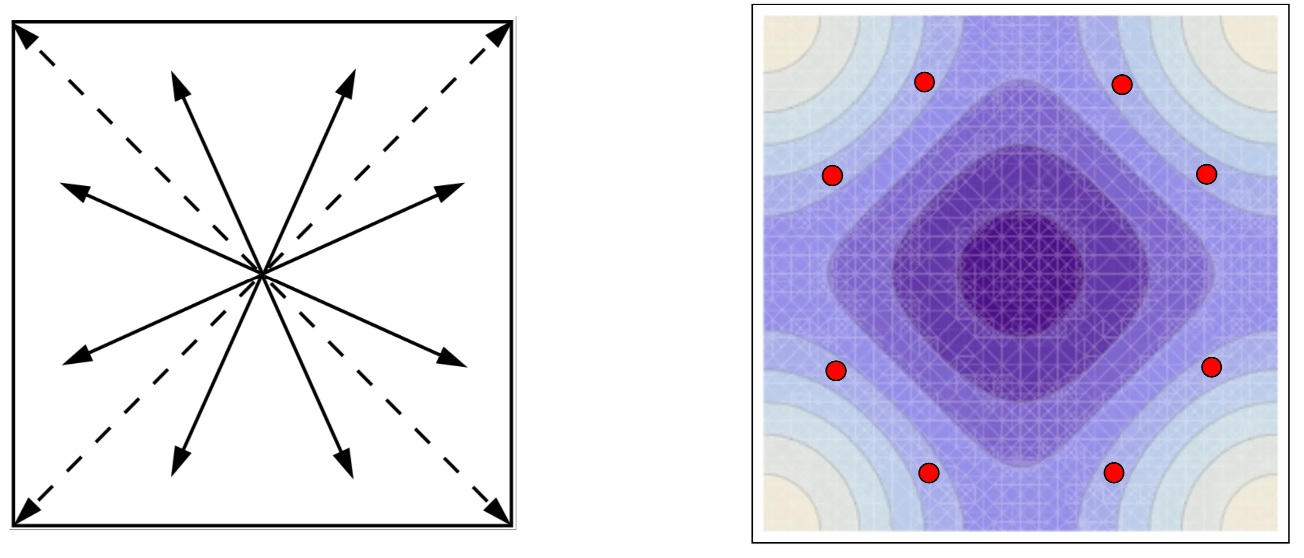
\begin{array}{r} ϵ_{g k} = ⟨ g k | H_{0} | g k ⟩ = ⟨ k | {\hat{S}}_{{g ∣ a}}^{- 1} H_{0} {\hat{S}}_{{g ∣ a}} | k ⟩ = ⟨ k | H_{0} | k ⟩ = ϵ_{k} . \end{array}

Consequently, there is a star-like structure of equivalent points $g k$ with the same band energy ( $\to$ degeneracy) for each $k$ in the Brillouin zone:

Attachments/Script 4.webp|700

This is called the 'star of $k$ -points' in the Brillouin zone with degenerate band energies: Left panel: Star of $k$ ; Right panel: contour plot of a two dimensional band $ϵ_{k}$ . The dots correspond to the star of $k$ points with degenerate energy values, demonstrating $ϵ_{n, k} = ϵ_{n, g k}$ .

For a general point $k$ the number of equivalent points in the star equals the number of point group elements for this $k$ (without inversion). If $k$ lies on points or lines of higher symmetry, it is left invariant under a subgroup of the point group. Consequently, the number of beams of the star is smaller. The subgroup of the point group leaving $k$ unchanged is called little group of $k$ . If inversion is part of the point group, $- k$ is always contained in the star of $k$ . In summary, we have the simple relations

\begin{array}{r} ϵ_{k} = ϵ_{g k}, ϵ_{k} = ϵ_{- k}, ϵ_{k} = ϵ_{k + G} \end{array}

Thus, we can also use symmetries to characterise Bloch states for given lattice momentum $k$ . We now extend our discussion to further symmetry aspects connected with the degeneracy of band energies. Consider the little group for given lattice momentum $k$ , which is generally a subgroup of the point group, $P_{k} \subset P$ . For the given $k$ we assume that there is a $d$ -fold degeneracy of the band energy $ϵ_{n, k}$ with states $| γ; n, k ⟩$ with $γ = 1, \dots, d$ , with

\begin{array}{r} H | γ; n, k ⟩ = ϵ_{n, k} | γ; n, k ⟩ and ⟨ γ; n, k ∣ γ^{'}; n, k ⟩ = δ_{γ γ^{'}} . \end{array}

Operating an element $g \in P_{k}$ yields again an eigenstate of $H$ with the same energy, because of $[H, {\hat{S}}_{{g, 0}}] = 0$ . Thus, we can write

\begin{array}{r} {\hat{S}}_{{g, 0}} | γ, n, k ⟩ = \sum_{γ^{'}} | γ^{'}, n, k ⟩ \underset{= M_{γ^{'}, γ} (g)}{\underset{⏟}{⟨ γ^{'}, n, k | {\hat{S}}_{{g, 0}} | γ, n, k ⟩}} \end{array}

where $M_{γ^{'}, γ} (g)$ is a $d \times d$ -matrix corresponding to the element $g$ and describing the transformation exclusively within the vector space defined by ${| γ; n, k ⟩}$ . The matrices $M_{γ^{'}, γ} (g)$ are a representation of $P_{k}$ in this vector space. If the degeneracy is symmetry-imposed and not accidental then this representation is even irreducible.

1.6 Band-Filling and Materials Properties

Due to the Fermionic character of electrons each of the band states $| n, k, s ⟩$ can be occupied with one electron taking also the spin quantum number into account with spin $s =↑$ and $↓$ (Pauli exclusion principle). The count of electrons has profound implications on the properties of materials. Here we would like to look at the most simple classification of materials based on independent electrons.

1.6.1 Electron Count and Band Filling

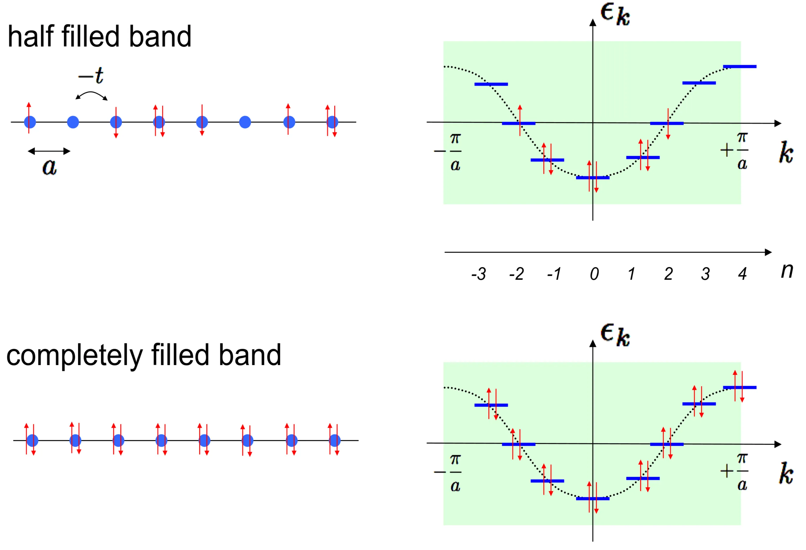
We consider here a most simple band structure in the one-dimensional tight-binding model with nearest-neighbour coupling. The lattice has $N$ sites ( $N$ even) and we assume periodic boundary conditions. The Hamiltonian is given by

\begin{array}{r} H = - t \sum_{j = 1}^{N} \sum_{s =↑, ↓} {{\hat{c}}_{j + 1, s}^{†} {\hat{c}}_{j, s} + {\hat{c}}_{j, s}^{†} {\hat{c}}_{j + 1, s}} \end{array}

where we impose the equivalence $j + N = j$ (periodic boundary conditions). This Hamiltonian can be diagonalised by the Fourier transform

\begin{array}{r} {\hat{c}}_{j, s} = \frac{1}{\sqrt{N}} \sum_{k} {\hat{a}}_{k, s} e^{i R_{j} k} \end{array}

leading to

\begin{array}{r} H = \sum_{k, s} ϵ_{k} {\hat{a}}_{k, s}^{†} {\hat{a}}_{k, s} with ϵ_{k} = - 2 t \cos k a . \end{array}

Now we request

\begin{aligned} e^{i R_{j} k} & = e^{i (R_{j} + L) k} \\ ⟹ L k & = N a k = 2 π n \\ ⟹ k & = \frac{2 π}{L} n = \frac{2 π}{a} \frac{n}{N} \end{aligned}

with the lattice momentum $k$ within the first Brillouin zone ( $- \frac{π}{a} < k < \frac{π}{a}$ ) and $n$ being an integer. On the real-space lattice an electron can take $2 N$ different states. Thus, for $k$ we find that $n$ should take the values, $n + N / 2 = 1, 2, \dots, N - 1, N$ . Note that $k = - π / a$ and $k = + π / a$ differ by a reciprocal lattice vector $G = 2 π / a$ and are therefore identical. This provides the same number of states ( $2 N$ ), since per $k$ we have two spins:

Attachments/Script 5.webp|700

We can fill these states with electrons following the Pauli exclusion principle. The figure shows the two typical situations:

$N$ electrons corresponding to half of the possible electrons which can be accommodated leading to a half-filled band, and
$2 N$ electrons exhausting all possible states representing a completely filled band. In the case of half-filling we define the Fermi energy as the energy $ϵ_{F}$ of the highest occupied state, here $ϵ_{F} = 0$ . This corresponds to the chemical potential, the energy necessary to add an electron to the system at $T = 0 K$ .

An important difference between 1. and 2. is that the former allows for many different states which may be separated from each other by a very small energy.

1.6.2 Metals, Semiconductors and Insulators

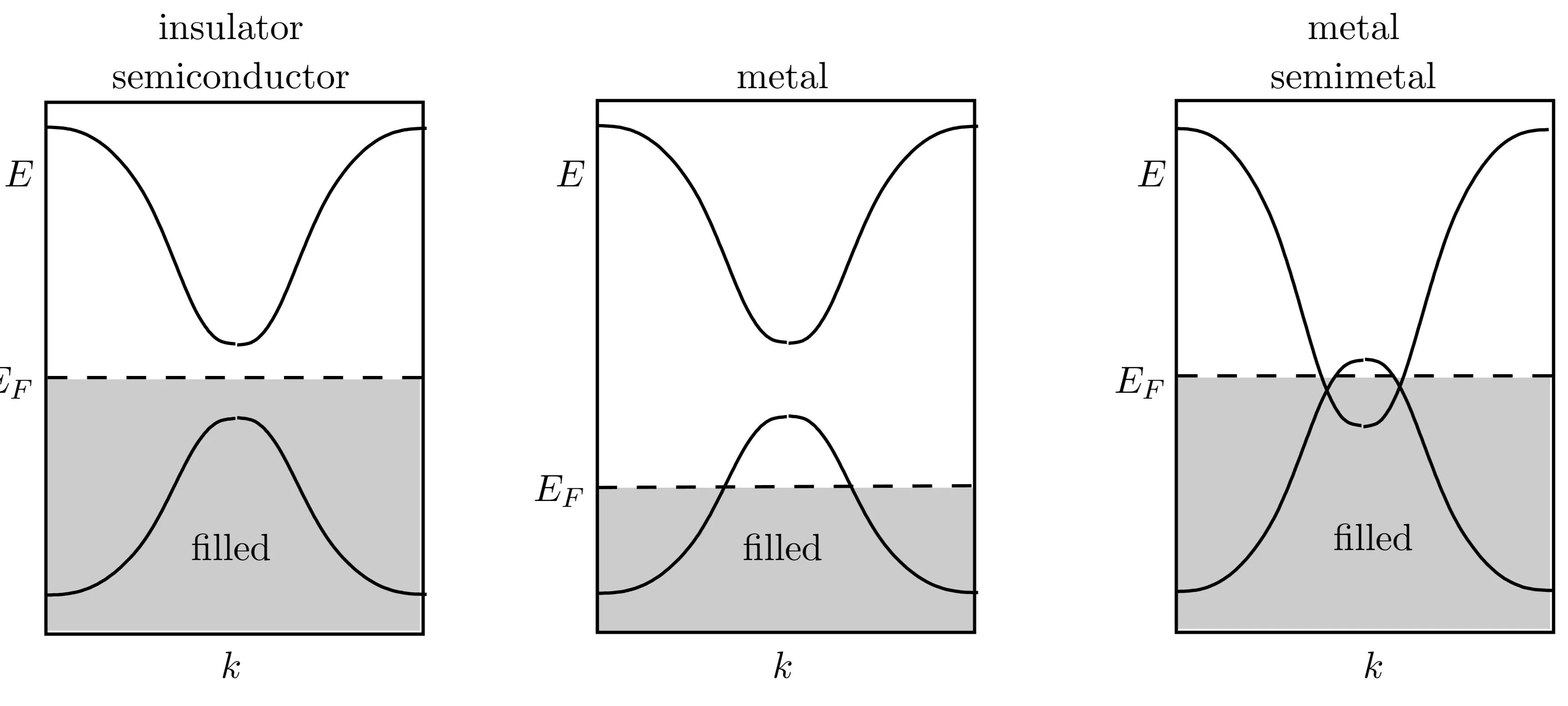
The two situations depicted in the next figure are typical as each atom (site) in a lattice contributes an integer number of electrons to the system. So we distinguish the case that there is an odd or an even number of electrons per unit cell. Note that the unit cell may contain more than one atom, unlike the situation shown in our tight-binding example.

In general, we make the distinction between different cases:

The bands can be either completely filled or empty when the number of electrons per atom (unit cell) is even. Thus taking the complete set of energy bands into account, the chemical potential cannot be identified with a Fermi energy but lies within the energy gap separating highest filled and the lowest empty band. There is a finite energy needed to add, to remove or to excite an electron. If the band gap $E_{g}$ is much smaller than the bandwidth, we call the material a semiconductor. For $E_{g}$ of the order of the bandwidth, it is an (band) insulator. In both cases, for temperatures $T ≪ E_{g} / k_{B}$ the application of a small electric voltage will not produce an electric transport. The highest filled band is called valence band, whereas the lowest empty band is termed conduction band. Examples for insulators are $C$ as diamond and for semiconductors $S i$ and $G e$ . They have diamond lattice structure with two atoms per unit cell. As these atoms belong to the group IV in the periodic table, each provides an even number of electrons suitable for completely filling bands. Note that we will encounter another form of an insulator, the Mott insulator, whose insulating behaviour is not governed by a band structure effect, but by a correlation effect through strong Coulomb interaction.
If the number of electrons per unit cell is odd, the uppermost non-empty band is half filled. Then the system is a metal, in which electrons can move and excitations with arbitrarily small energies are possible. The electrons remain mobile down to arbitrarily low temperatures. The standard example of a metal are the Alkali metals in the first column of the periodic table (Li, Na, K, Rb, Cs), as all of them have the configuration [noble gas] $(n s)^{1}$ , that is, one mobile electron per ion.
In general, band structures are more complex. Different bands need not to be separated by energy gaps, but can overlap instead. In particular, this happens, if different orbitals are involved in the structure of the bands. In these systems, bands can have any fractional filling (not just filled or half-filled). The earth alkaline metals are an example for this (second column of the periodic table, Be, Mg, Ca, Sr, Ba), which are metallic despite having two ( $n s$ )-electrons per unit cell. Systems, where two bands overlap at the Fermi energy but the overlap is small, are termed semi-metals. The extreme case, where valence and conduction band touch in isolated points so that there are no electrons at the Fermi energy and still the band gap is zero, is realised in graphene.

Attachments/Script 6.webp|700
The electronic structure is also responsible for the cohesive forces necessary for the formation of a regular crystal. We may also classify materials according to relevant forces. We distinguish four major types of crystals:

Molecular crystals are formed from atoms or molecules with closed-shell atomic structures such as the noble gases He, Ne, etc. which become solid under pressure. Here the van der Waals forces generate the binding interactions.

Ionic crystals combine different atoms, A and B, where A has a small ionisation energy while B has a large electron affinity. Thus, electrons are transferred from A to B giving a positively charged $A^{+}$ and a negatively charge $B^{-}$ . In a regular (alternating) lattice the energy gained through Coulomb interaction can overcome the energy expense for the charge transfer stabilising the crystal. A famous example is NaCl where one electron leaves Na ([Ne] $3 s$ ) and is added to Cl ([Ne] $3 s^{2} 3 p^{5}$ ) as to bring both atoms to closed-shell electronic configuration.

Covalent-bonded crystals form through chemical binding, like in the case of the $H_{2}$ , where neighboring atoms share electrons through the large overlap of the electron orbital wavefunction. Insulators like diamond C or semiconductors like Si or GaAs are important examples of this type as we will discuss later. Note that electrons of covalent bonds are localised between the atoms.

Metallic bonding is based on delocalised electrons (in contrast to the covalent bonds) stripped from their atoms. The stability of simple metals like the alkali metals Li, Na, K etc will be discussed later. Note that many metals, such as the noble metals Au or Pt can also involve aspects of covalent or molecular bonding through overlapping but more localised electronic orbitals.

1.7 Dynamics of Band Electrons - Semiclassical Approach

In quantum mechanics, the Ehrenfest theorem shows that the expectation values of the position and momentum operators obey equations similar to the equation of motion in Newtonian mechanics. An analogous formulation holds for electrons in a periodic potential, where we assume that the electron may be described as a wave packet of the form

\begin{array}{r} ψ_{k} (r, t) = \sum_{k^{'}} g_{k} (k^{'}) e^{i k^{'} \cdot r - i ϵ_{k^{'}} t / ℏ} \end{array}

where $g_{k} (k^{'})$ is centred around $k$ in reciprocal space and has a width of $Δ k . Δ k$ should be much smaller than the size of the Brillouin zone for this Ansatz to make sense, that is, $Δ k ≪ 2 π / a$ . Therefore, the wave packet is spread over many unit cells of the lattice since Heisenberg's uncertainty principle $(Δ k) (Δ x) > 1$ implies $Δ x ≫ a / 2 π$ . In this way, the lattice momentum $k$ of the wave packet remains well defined. Furthermore, the applied electric and magnetic fields have to be small enough not to induce transitions between different bands. The latter condition is not very restrictive in practice.

1.7.1 Semi-Classical Equations of Motion

We introduce the rules of the semi-classical motion of electrons with applied electric and magnetic fields without proof:

The band index of an electron is conserved, that is, there are no transitions between the bands.
The equations of motion read

\begin{aligned} \dot{r} & = v_{n} (k) = \frac{\partial ϵ_{n k}}{\partial ℏ k}, \\ ℏ \dot{k} & = - e E (r, t) - \frac{e}{c} v_{n} (k) \times H (r, t) . \end{aligned}

All electronic states have a wave vector that lies in the first Brillouin zone, as $k$ and $k + G$ label the same state for all reciprocal lattice vectors $G$ .
In thermal equilibrium, the electron density per spin in the $n$ -th band in the volume element $d^{3} k / (2 π)^{3}$ around $k$ is given by

n_{F} [ϵ_{n} (k)] = \frac{1}{e^{[ϵ_{n} (k) - μ] / k_{B} T} + 1} .

Each state of given $k$ and spin can be occupied only once (Pauli principle).

Note that $ℏ k$ is not the momentum of the electron, but the so-called lattice momentum or crystal momentum in the Bloch theory of bands. It is connected with the eigenvalue of the translation operator on the state. Consequently, the right-hand side of the equation for the time evolution of the lattice momentum is not the total force that acts on the electron, as the forces exerted by the periodic lattice potential are not included. The latter effect is contained implicitly through the form of the band energy $ϵ (k)$ , which governs the first equation of motion.

1.7.2 Bloch Oscillations

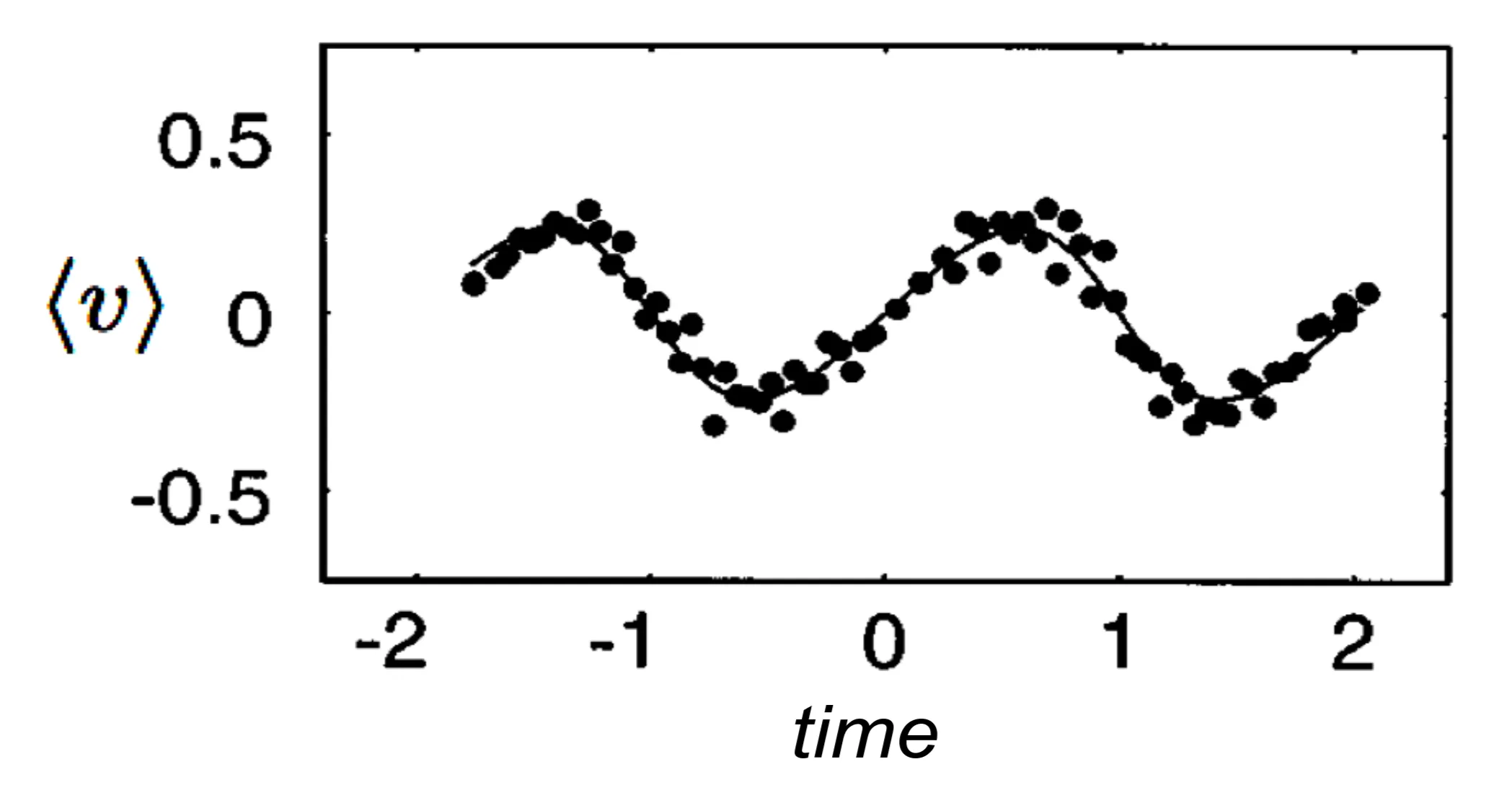
The fact that the band energy is a periodic function of $k$ leads to a strange oscillatory behaviour of the electron motion in a static electric field. For illustration, consider a one-dimensional system where the band energy $ϵ_{k} = - 2 t \cos k a$ leads to the solution of the semi-classical equations:

\begin{aligned} ℏ \dot{k} & = - e E \\ ⟹ k & = - \frac{e E t}{ℏ} \\ ⟹ \dot{x} & = - \frac{2 a t}{ℏ} \sin (\frac{e E a t}{ℏ}), \end{aligned}

in the presence of a homogenous electric field $E$ . It follows immediately, that the position $x$ of the electron oscillates like

\begin{array}{r} x (t) = \frac{2 t}{e E} \cos (\frac{e E a t}{ℏ}) . \end{array}

This behaviour is called Bloch oscillation and means that the electron oscillates around its initial position rather than moving in one direction when subjected to a static electric field. This effect can only be observed under very special conditions where the probe is absolutely clean. The effect is easily destroyed by damping or scattering, but has been experimentally observed for accelerated caesium atoms:

Attachments/Script 7.webp|700

1.7.3 Current Densities

We will see in a later chapter that homogenous steady current carrying states of electron systems can be described by the momentum distribution $n (k)$ . Assuming this property, the current density follows from

\begin{array}{r} j = - 2 e \int_{BZ} \frac{d^{3} k}{(2 π)^{3}} v (k) n (k) = - 2 e \int_{BZ} \frac{d^{3} k}{(2 π)^{3}} n (k) \frac{\partial ϵ (k)}{\partial ℏ k}, \end{array}

where the integral extends over all $k$ in the Brillouin zone (BZ) and the factor 2 originates from the two possible spin states of the electrons. Note that for a finite current density $j$ , the momentum distribution $n (k)$ has to deviate from the equilibrium Fermi-Dirac distribution previously mentioned. It is straightforward to show that the current density vanishes for an empty band. The same holds true for a completely filled band ( $n (k) = 1$ ), where the definition of group velocity implies

\begin{array}{r} j = - 2 e \int_{BZ} \frac{d^{3} k}{(2 π)^{3}} \frac{1}{ℏ} \frac{\partial ϵ (k)}{\partial k} = 0 \end{array}

because $ϵ (k)$ is periodic in the Brillouin zone, that is, $ϵ (k + G) = ϵ (k)$ when $G$ is a reciprocal lattice vector. Thus, neither empty nor completely filled bands can carry currents.
An interesting aspect of band theory is the picture of holes. We compute the current density for a partially filled band in the framework of the semi-classical approximation,

\begin{aligned} j & = - 2 e \int_{BZ} \frac{d^{3} k}{(2 π)^{3}} n (k) v_{n} (k) \\ = - 2 e [\int_{BZ} \frac{d^{3} k}{(2 π)^{3}} v (k) - \int_{BZ} \frac{d^{3} k}{(2 π)^{3}} [1 - n (k)] v (k)] \\ = + 2 e \int_{BZ} \frac{d^{3} k}{(2 π)^{3}} [1 - n (k)] v (k) . \end{aligned}

This suggests that the current density comes either from electrons in filled states with charge $- e$ or from 'holes', missing electrons carrying positive charge and sitting in the unoccupied electronic states. In band theory, both descriptions are equivalent. However, it is usually easier to work with holes, if a band is almost filled, and with electrons if the filling of an energy band is small.

1.8 Approximative Band Structure Calculations

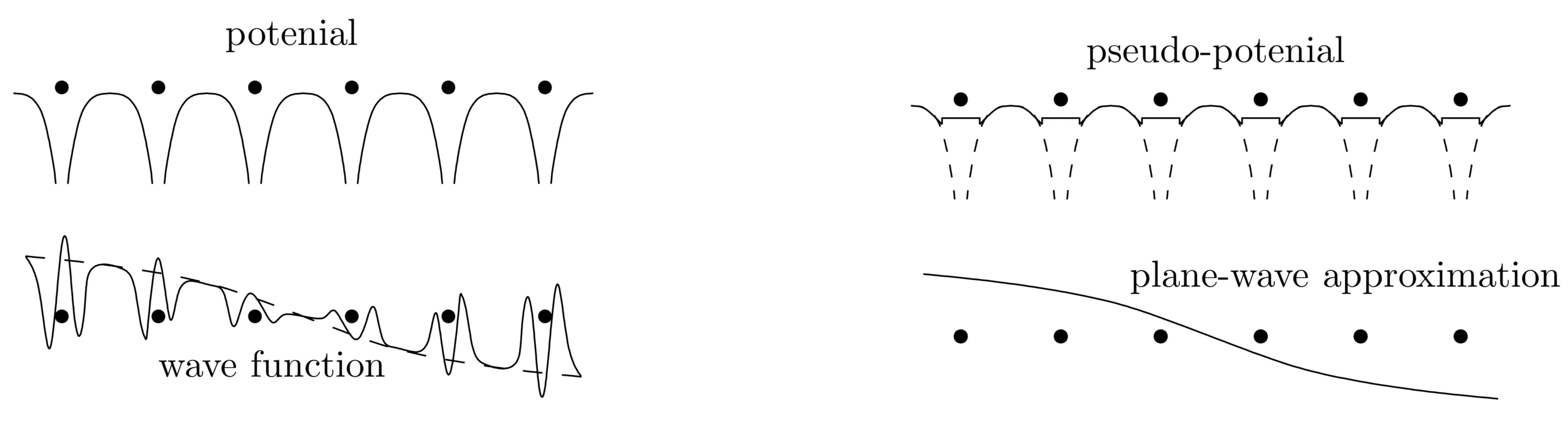
While the approximation of nearly free electrons gives a qualitative picture of the band structure, it rests on the assumption that the periodic potential is weak, and, thus, may be treated as a small perturbation. Only few states connected with different reciprocal lattice vectors are sufficient within this approximation. However, in reality the ionic potential is strong compared to the electrons' kinetic energy. This leads to strong modulations of the wave function around the ions, which is not well described by slightly perturbed plane waves.

1.8.1 Pseudo-Potential

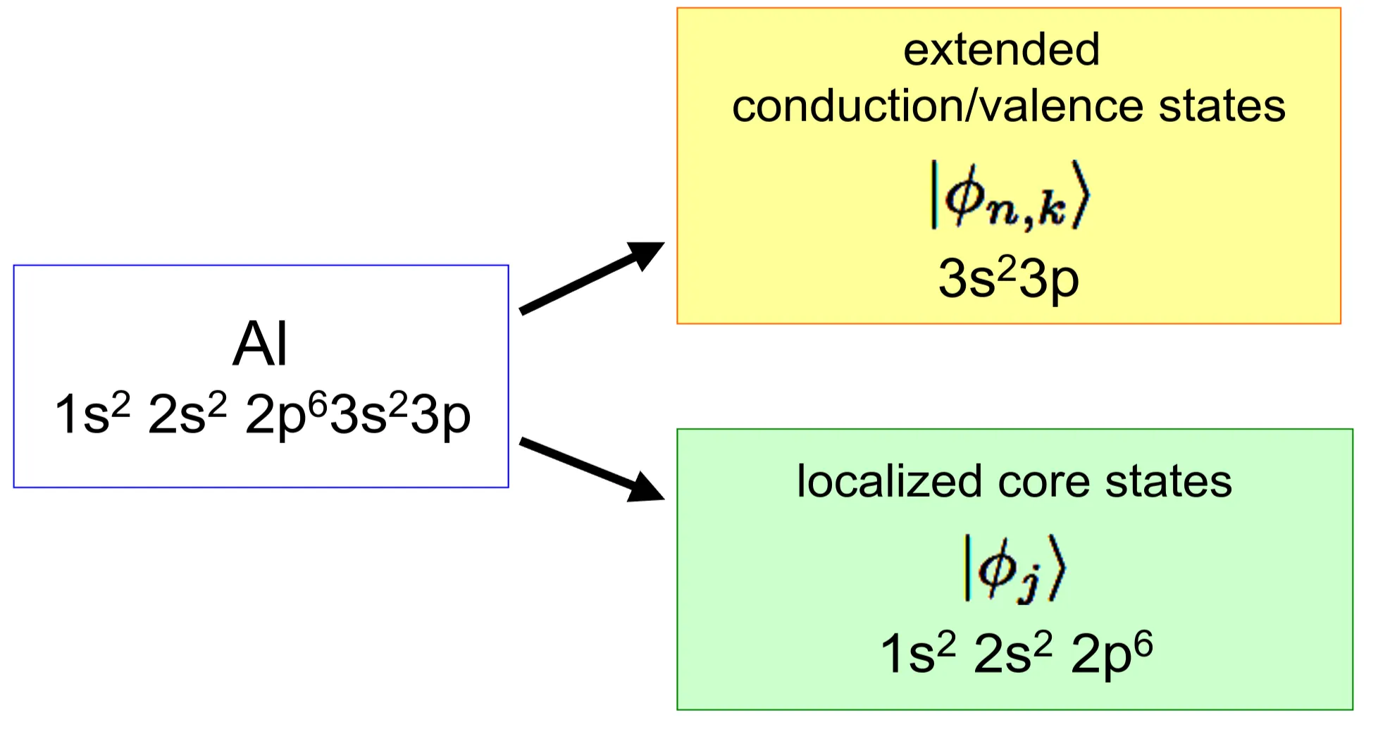
In order to overcome this weakness of the plane wave solution, we would have to superpose a very large number of plane waves, which is not an easy task to put into practice. Alternatively, we can divide the electronic states into the ones corresponding to filled low-lying energy states, which are concentrated around the ionic core (core states), and into extended (and more weakly modulated) states, which form the valence and conduction bands. The core electron states may be approximated by atomic orbitals of isolated atoms. For a metal such as aluminium (Al: $1 s^{2} 2 s^{2} 2 p^{6} 3 s^{2} 3 p$ ) the core electrons correspond to the $1 s$ -, $2 s$ -, and $2 p$ -orbitals, whereas the $3 s$ and $3 p$ -orbitals contribute dominantly to the extended states of the valence- and conduction bands. We will focus on the latter, as they determine the low-energy physics of the electrons. The core electrons are deeply bound and can be considered inert.

Attachments/Script 8.webp|700

We introduce the core electron states as $| ϕ_{j} ⟩$ , with $H | ϕ_{j} ⟩ = E_{j} | ϕ_{j} ⟩$ where $H$ is the Hamiltonian of the single atom. The remaining states have to be orthogonal to these core states, so that we make the Ansatz

\begin{array}{r} | ϕ_{n, k} ⟩ = | χ_{n k} ⟩ - \sum_{j} | ϕ_{j} ⟩ ⟨ ϕ_{j} ∣ χ_{n, k} ⟩, \end{array}

with $| χ_{n k} ⟩$ an orthonormal set of states. Then, $⟨ ϕ_{n, k} ∣ ϕ_{j} ⟩ = 0$ holds for all $j$ . If we choose plane waves for the $| χ_{n k} ⟩$ , the resulting $| ϕ_{n, k} ⟩$ are so-called orthogonalised plane waves (OPW).

The Bloch functions are superpositions of these OPW,

\begin{array}{r} | ψ_{n, k} ⟩ = \sum_{G} b_{k + G} | ϕ_{n, k + G} ⟩ \end{array}

where the coefficients $b_{k + G}$ converge rapidly, such that, hopefully, only a small number of OPWs is needed for a good description.
First, we again consider an arbitrary $| χ_{n k} ⟩$ and insert it into the eigenvalue equation $H | ϕ_{n k} ⟩ = E_{n k} | ϕ_{n k} ⟩$ ,

\begin{array}{r} H | χ_{n k} ⟩ - \sum_{j} H | ϕ_{j} ⟩ ⟨ ϕ_{j} ∣ χ_{n, k} ⟩ = E_{n k} (| χ_{n k} ⟩ - \sum_{j} | ϕ_{j} ⟩ ⟨ ϕ_{j} ∣ χ_{n, k} ⟩) \end{array}

\begin{array}{r} H | χ_{n k} ⟩ + \sum_{j} (E_{n k} - E_{j}) | ϕ_{j} ⟩ ⟨ ϕ_{j} ∣ χ_{n, k} ⟩ = E_{n k} | χ_{n k} ⟩ . \end{array}

We introduce the integral operator in real space ${\hat{V}}^{'} = \sum_{j} (E_{n k} - E_{j}) | ϕ_{j} ⟩ ⟨ ϕ_{j} |$ , describing a non-local and energy-dependent potential. With this operator we can rewrite the eigenvalue equation in the form

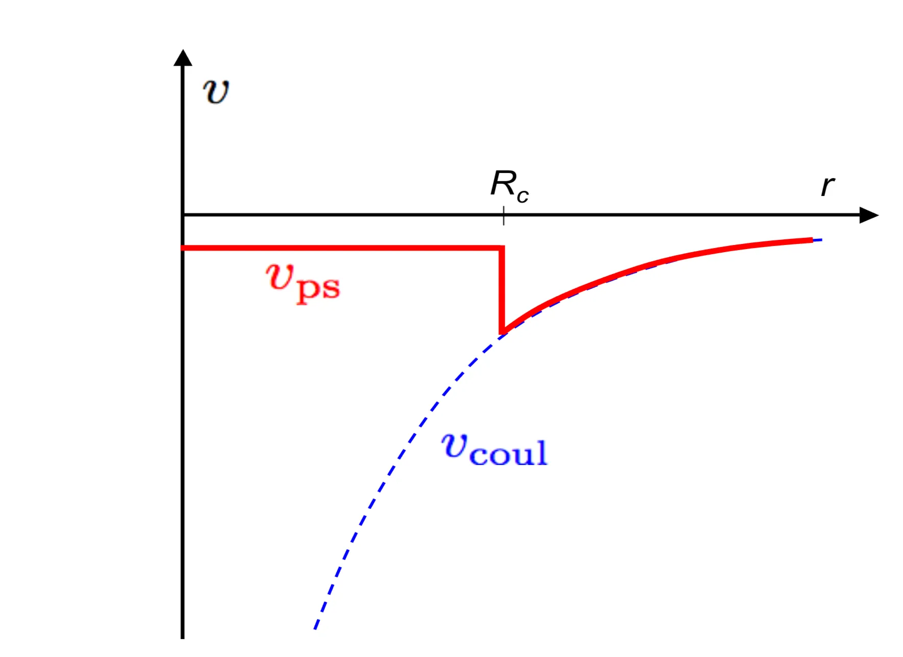
\begin{aligned} (H + {\hat{V}}^{'}) | χ_{n, k} ⟩ & = (H_{0} + \hat{V} + {\hat{V}}^{'}) | χ_{n, k} ⟩ \\ = (H + {\hat{V}}_{ps}) | χ_{n, k} ⟩ = E_{n k} | χ_{n k} ⟩ \end{aligned}

This is an eigenvalue equation for the so-called pseudo-wave function (or pseudo-state) $| χ_{n k} ⟩$ , instead of the Bloch state $| ψ_{n k} ⟩$ , where the modified potential ${\hat{V}}_{ps} = \hat{V} + {\hat{V}}^{'}$ is called pseudopotential. The attractive core potential $\hat{V} = V (\hat{r})$ is always negative. On the other hand, $E_{n k} > E_{j}$ , such that ${\hat{V}}^{'}$ is positive. It follows that ${\hat{V}}_{ps}$ is weaker than both $\hat{V}$ and ${\hat{V}}^{'}$ . An arbitrary number of core states $\sum_{j} a_{j} | ψ_{j} ⟩$ may be added to $| χ_{n k} ⟩$ without violating the orthogonality condition between valence and core states. Consequently, neither the pseudo-potential nor the pseudo-states are uniquely determined and may be optimised variationally with respect to the set ${a_{j}}$ in order to optimally reduce the spatial modulation of either the pseudo-potential or the wave-function.

Attachments/Script 9.webp|700

If we are only interested in states inside a small energy window, the energy dependence of the pseudo-potential can be neglected, and $V_{ps}$ may be approximated by a standard potential. Such a simple Ansatz is exemplified by the atomic pseudo-potential, proposed by Ashcroft, Heine and Abarenkov (AHA). The potential of a single ion is assumed to be of the form

\begin{array}{r} v_{ps} (r) = {\begin{cases} V_{0} & r < R_{c} \\ - \frac{Z_{ion} e^{2}}{r} & r > R_{c} \end{cases} \end{array}

where $Z_{ion}$ is the charge of the ionic core and $R_{c}$ its effective radius (determined by the core electrons). The constants $R_{c}$ and $V_{0}$ are chosen such that the energy levels of the outermost electrons are reproduced correctly for the single-atom calculations.

Attachments/Script 10.webp|700

For example, the $1 s$ -, $2 s$ -, and $2 p$ -electrons of Na form the ionic core. $R_{c}$ and $V_{0}$ are adjusted such that the one-particle problem $p^{2} / 2 m + v_{ps} (r)$ leads to the correct ionisation energy of the $3 s$ -electron. More flexible approaches allow for the incorporation of more experimental input into the pseudo-potential. The full pseudo-potential of the lattice can be constructed from the contribution of the individual atoms,

\begin{array}{r} V_{ps} (r) = \sum_{j} v_{ps} (| r - R_{j} |), \end{array}

where $R_{j}$ is the lattice vector. For the method of nearly free electrons we need the Fourier transform of the potential evaluated at the reciprocal lattice vectors,

\begin{array}{r} V_{ps, G} = \frac{1}{Ω} \int d^{3} r V_{ps} (r) e^{- i G \cdot r} = \frac{N}{Ω} \int d^{3} r v_{ps} (| r |) e^{- i G \cdot r} . \end{array}

For the AHA form, this is given by

\begin{aligned} V_{ps, G} & = - \frac{4 π Z_{ion} e^{2}}{G^{2}} \cos (G R_{c}) \\ + \frac{V_{0}}{Z_{ion} e^{2} G} ((R_{c}^{2} G^{2} - 2) \cos (G R_{c}) + 2 - 2 R_{c} G \sin (G R_{c})) . \end{aligned}

For small reciprocal lattice vectors, the zeroes of the trigonometric functions on the right-hand side of the expression for $V_{ps, G}$ reduce the strength of the potential. For large $G$ , the pseudo-potential decays $\sim 1 / G^{2}$ . It is thus clear that the pseudo-potential is always weaker than the original potential. Extending this theory for complex unit cells containing more than one atom, the pseudo-potential may be written as

\begin{array}{r} V_{ps} (r) = \sum_{j, α} v_{ps}^{α} (| r - (R_{j} + R_{α}) |), \end{array}

where $R_{α}$ denotes the position of the $α$ -th base atom in the unit cell. Here, $v_{ps}^{α}$ is the pseudopotential of the $α$ -th ion. In reciprocal space,

\begin{aligned} V_{ps, G} & = \frac{N}{Ω} \sum_{α} e^{- i G \cdot R_{α}} \int d^{3} r v_{ps}^{α} (| r |) e^{- i G \cdot r} \\ = \sum_{α} e^{- i G \cdot R_{α}} F_{α, G} \end{aligned}

The form factor $F_{α, G}$ contains the information of the base atoms and may be calculated or obtained by fitting experimental data.

1.8.2 Augmented Plane Wave

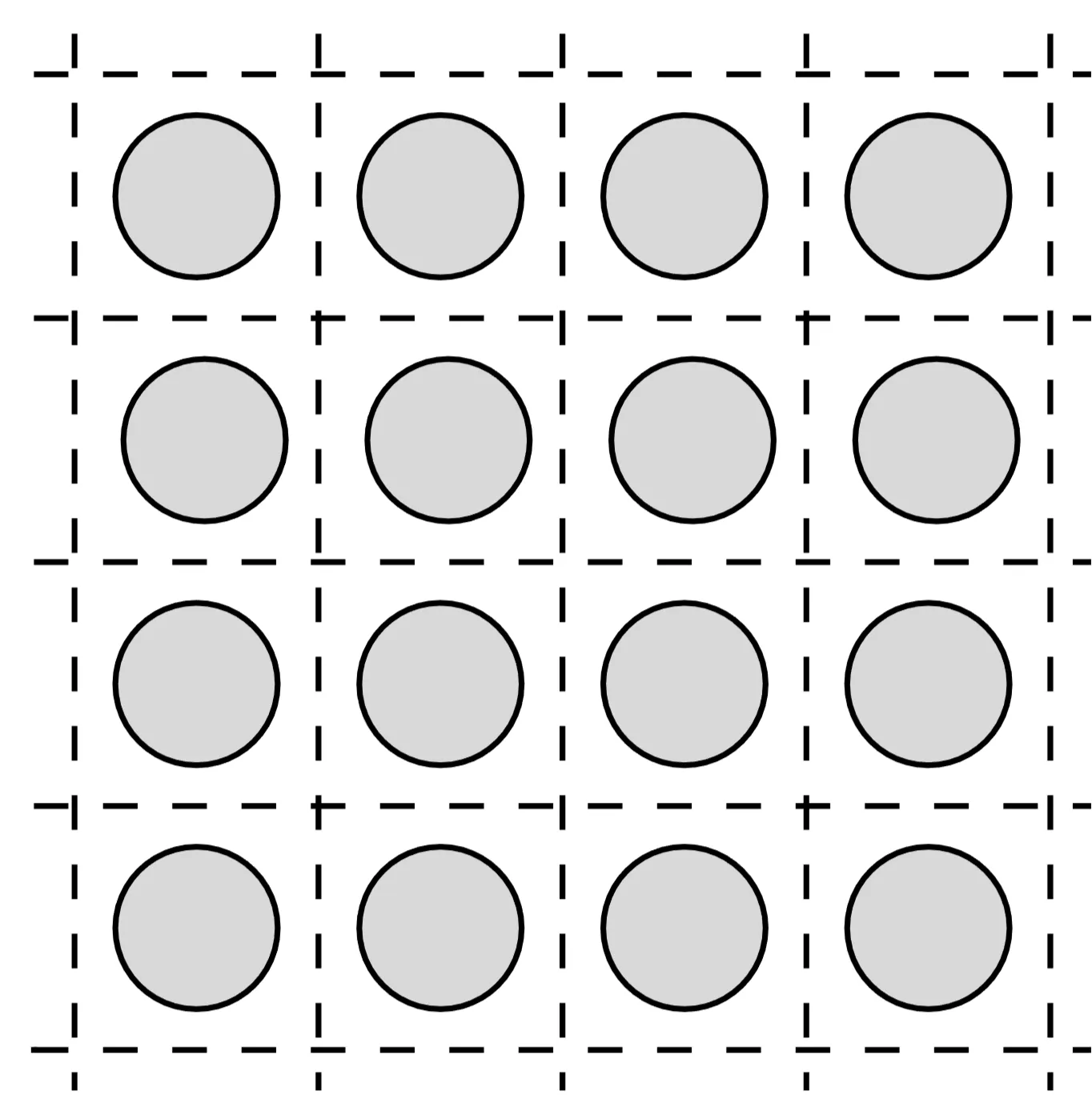
We now consider a method introduced by Slater in 1937. It is an extension of the so-called Wigner-Seitz cell method (1933) and consists of approximating the crystal potential by a so-called muffin-tin potential. The latter is a periodic potential, which is taken to be spherically symmetric and position dependent around each atom up to a distance $r_{s}$ , and constant for larger distances. The spheres of radius $r_{s}$ are taken to be non-overlapping and are contained completely in the Wigner-Seitz cell:

Attachments/Script 11.webp|700

The advantage of this decomposition is that the problem can be solved using a divide-and-conquer strategy. Inside the muffin-tin radius we solve the spherically symmetric problem, while the solutions on the outside are given by plane waves; the remaining task is to match the solutions at the boundaries.
The spherically symmetric problem for $| r | < r_{s}$ is solved with the standard Ansatz

\begin{array}{r} φ (r) = \frac{u_{l} (r)}{r} Y_{l m} (θ, ϕ), \end{array}

where $(r, θ, ϕ)$ are the spherical coordinates of $r$ and the radial part $u_{l} (r)$ of the wave function obeys the differential equation

\begin{array}{r} [- \frac{ℏ^{2}}{2 m} \frac{d^{2}}{d r^{2}} + \frac{ℏ^{2} l (l + 1)}{2 m r^{2}} + V (r) - E] u_{l} (r, E) = 0 . \end{array}

We define an augmented plane wave (APW) $A (k, r, E)$ , which is a pure plane wave with wave vector $k$ outside the Muffin-tin sphere. For this, we employ the representation of plane waves by spherical harmonics,

\begin{array}{r} e^{i k \cdot r} = 4 π \sum_{l = 0}^{\infty} \sum_{m = - l}^{l} i^{l} j_{l} (k r) Y_{l m}^{*} (\hat{k}) Y_{l m} (\hat{r}), \end{array}

where $j_{l} (x)$ is the $l$ -th spherical Bessel function, $k = | k |$ , $r = | r |$ , and $\hat{k}, \hat{r}$ are unit vectors. We parametrise

\begin{array}{r} A (k, r, E) = {\begin{cases} \frac{4 π}{\sqrt{Ω_{UC}}} \sum_{l, m} i^{l} j_{l} (k r_{s}) \frac{r_{s} u_{l} (r, E)}{r u_{l} (r_{s}, E)} Y_{l m}^{*} (\hat{k}) Y_{l m} (\hat{r}), & r < r_{s}, \\ \frac{4 π}{\sqrt{Ω_{UC}}} \sum_{l, m} i^{l} j_{l} (k r) Y_{l m}^{*} (\hat{k}) Y_{l m} (\hat{r}), & r > r_{s} \end{cases} \end{array}

where $Ω_{UC}$ is the volume of the unit cell. Note that the wave function is always continuous at $r = r_{s}$ , but that its derivatives are in general not continuous. We can use an expansion of the wave function $ψ_{k} (r)$ similar to one seen previously in the nearly free electron approximation,

\begin{array}{r} ψ_{k} (r) = \sum_{G} c_{G} (k) A (k + G, r, E) \end{array}

where the $G$ are reciprocal lattice vectors. The unknown coefficients can be determined variationally by solving the system of equations

\begin{array}{r} \sum_{G} ⟨ A_{k} (E) | H - E | A_{k + G} (E) ⟩ c_{G} (k) = 0, \end{array}

where

\begin{array}{r} ⟨ A_{k} (E) | H - E | A_{k^{'}} (E) ⟩ = (\frac{ℏ^{2} k \cdot k^{'}}{2 m} - E) Ω_{UC} δ_{k, k^{'}} + V_{k, k^{'}} \end{array}

with

\begin{aligned} V_{k, k^{'}} = 4 π r_{s}^{2} [- (\frac{ℏ^{2} k \cdot k^{'}}{2 m} - E) & \frac{j_{1} (| k - k^{'} | r_{s})}{| k - k^{'} |} \\ + \sum_{l = 0}^{\infty} \frac{ℏ^{2}}{2 m} (2 l + 1) P_{l} (\hat{k} \cdot {\hat{k}}^{'}) j_{l} (k r_{s}) j_{l} (k^{'} r_{s}) \frac{u_{l}^{'} (r_{s}, E)}{u_{l} (r_{s}, E)}] . \end{aligned}

Here, $P_{l} (z)$ is the $l$ -th Legendre polynomial and $u^{'} = d u / d r$ . The solution of this system of equations yields the energy bands. The most difficult parts are the approximation of the crystal potential by the muffin-tin potential and the computation of these matrix elements. The rapid convergence of the method is its big advantage: just a few dozens of $G$ -vectors are needed and the largest angular momentum needed is about $l = 5$ . Another positive aspect is the fact that the APW-method allows the interpolation between the two extremes of extended, weakly bound electronic states and tightly bound states.