5 Discrete-Time Fourier Transform

5.1 Representation of Aperiodic Signals: The Discrete-Time Fourier Transform

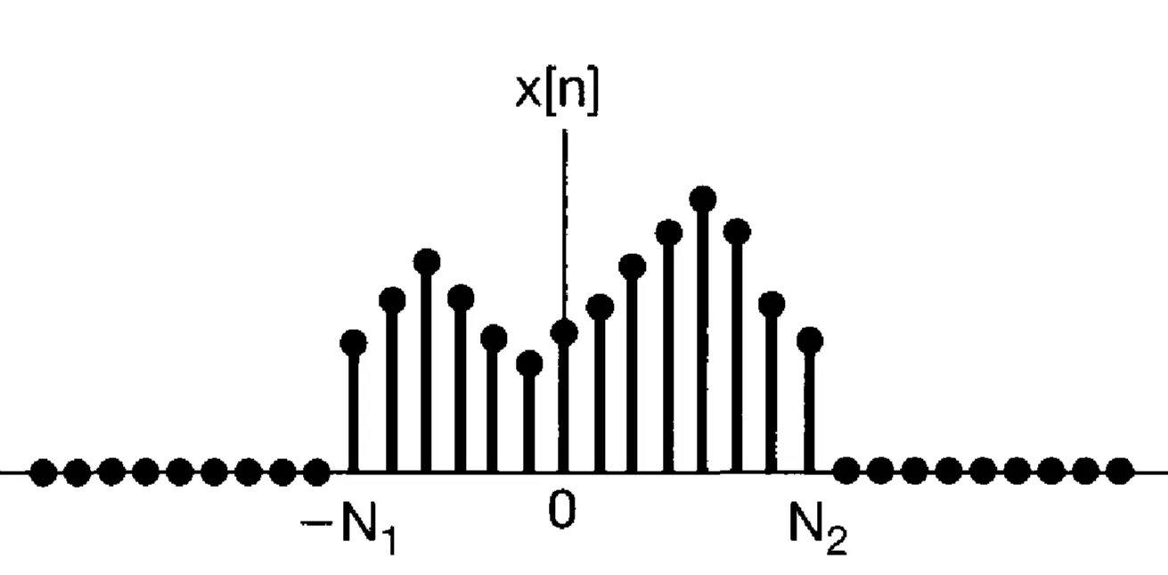
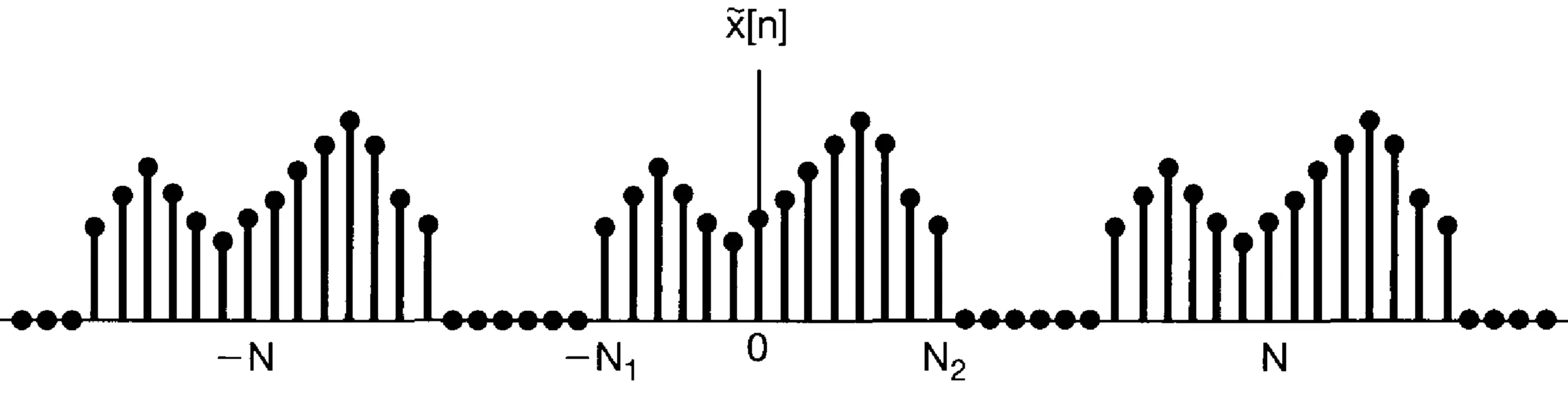
Consider a general aperiodic sequence $x [n]$ . For heuristic derivation, we can initially imagine $x [n]$ as being of finite duration, such that $x [n] = 0$ outside some range, for instance $N_{1} \leq n \leq N_{2}$ . From this aperiodic signal, we can construct a periodic signal $\tilde{x} [n]$ by repeating $x [n]$ with a period $N > (N_{2} - N_{1} + 1)$ , so that the original $x [n]$ (padded with zeros to length $N$ if necessary) forms one period of $\tilde{x} [n]$ :

Attachments/Oppenheim,Willsky_Signals and Systems 20.webp|700

As we increase the period $N \to \infty$ , the periodic signal $\tilde{x} [n]$ becomes identical to the aperiodic signal $x [n]$ for all $n$ . By considering the Discrete-Time Fourier Series (DTFS) of $\tilde{x} [n]$ and taking this limit, we can derive the Discrete-Time Fourier Transform (DTFT) pair:

Synthesis (Inverse DTFT): x [n] = \frac{1}{2 π} \int_{2 π} X (e^{i ω}) e^{i ω n} d ω,

Analysis (Forward DTFT): X (e^{i ω}) = \sum_{n = - \infty}^{+ \infty} x [n] e^{- i ω n} .

The function $X (e^{i ω})$ is the Fourier transform of $x [n]$ , often called its spectrum. A key property of $X (e^{i ω})$ is that it is always periodic in $ω$ with period $2 π$ , i.e., $X (e^{i (ω + 2 π)}) = X (e^{i ω})$ . Consequently, the integral in the synthesis equation can be evaluated over any interval of length $2 π$ , commonly $[0, 2 π]$ or $[- π, π]$ .

Compared to the continuous-time Fourier transform (CTFT), where the spectrum $X (i Ω)$ is generally aperiodic, the discrete-time spectrum $X (e^{i ω})$ is always periodic. The synthesis integral for DTFT is also over a finite frequency interval, whereas for CTFT it is over an infinite interval. The periodicity of $X (e^{i ω})$ arises because discrete-time complex exponentials $e^{i ω n}$ are themselves periodic in $ω$ with period $2 π$ (since $e^{i (ω + 2 π) n} = e^{i ω n} e^{i 2 π n} = e^{i ω n}$ for integer $n$ ).

A consequence of this $2 π$ -periodicity is that frequencies $ω$ and $ω + 2 π m$ (for any integer $m$ ) are indistinguishable for discrete-time signals. Low frequencies (slowly varying signals $x [n]$ ) correspond to values of $ω$ near integer multiples of $2 π$ (for example, $ω \approx 0, \pm 2 π, \dots$ ). High frequencies (rapidly varying signals $x [n]$ ) correspond to values of $ω$ near odd multiples of $π$ (for example, $ω \approx \pm π, \pm 3 π, \dots$ ; $e^{i π n} = (- 1)^{n}$ is the most rapidly varying sequence). This behaviour is illustrated below:

Attachments/Oppenheim,Willsky_Signals and Systems 22.webp|700

5.1.1 Convergence Issues of the Discrete-Time Fourier Transform

The derivation above heuristically assumed a finite-duration $x [n]$ . However, the DTFT pair also holds for many signals of infinite duration. For the infinite summation in the analysis equation $X (e^{i ω}) = \sum_{n = - \infty}^{+ \infty} x [n] e^{- i ω n}$ to converge, $x [n]$ must satisfy certain conditions. Sufficient conditions include:

$x [n]$ is absolutely summable: $\sum_{n = - \infty}^{+ \infty} | x [n] | < \infty .$ If this holds, $X (e^{i ω})$ converges uniformly to a continuous function of $ω$ .
$x [n]$ has finite energy (is square-summable): $\sum_{n = - \infty}^{+ \infty} | x [n] |^{2} < \infty .$ If this holds, $X (e^{i ω})$ converges in the mean-square sense over one period.

These conditions are analogous to those for the continuous-time Fourier transform. Notably, the inverse transform integral (synthesis equation) always converges if $X (e^{i ω})$ is a valid DTFT that is, for instance, square-integrable over one period, because the integration is over a finite interval.

5.2 The Fourier Transform for Periodic Signals

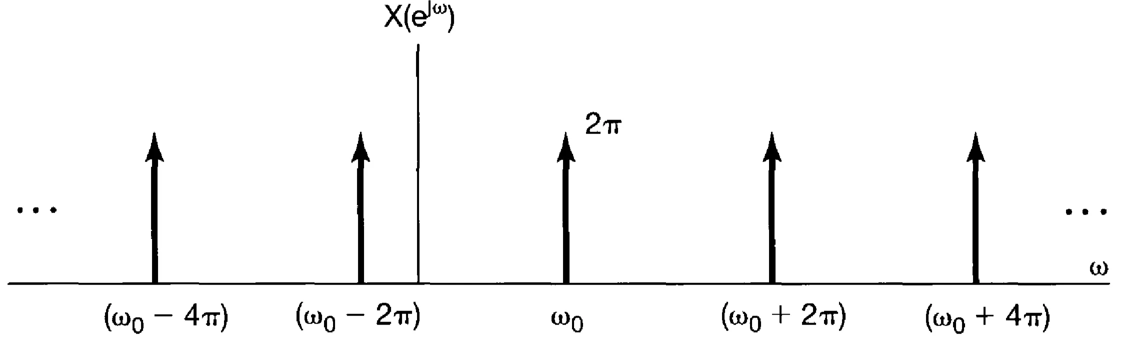
As in the continuous-time case, the DTFT can be extended to include periodic signals by allowing Dirac impulse functions in the frequency domain representation. Consider a single complex exponential sequence:

x [n] = e^{i ω_{0} n} .

In continuous time, the Fourier transform of $e^{i ω_{0} t}$ is $2 π δ (ω - ω_{0})$ . For discrete time, due to the $2 π$ -periodicity of the DTFT spectrum, we expect a periodic train of impulses:

X (e^{i ω}) = \sum_{l = - \infty}^{+ \infty} 2 π δ (ω - ω_{0} - 2 π l) .

This represents impulses at $ω_{0}, ω_{0} \pm 2 π, ω_{0} \pm 4 π, \dots$ .

Attachments/Oppenheim,Willsky_Signals and Systems 23.webp|700

To verify, the inverse DTFT over any interval of length $2 π$ (which will contain exactly one impulse from the train, say at $ω_{0} + 2 π r$ for some integer $r$ ) gives:

\begin{aligned} \frac{1}{2 π} \int_{2 π} X (e^{i ω}) e^{i ω n} d ω & = \frac{1}{2 π} \int_{2 π} (\sum_{l = - \infty}^{+ \infty} 2 π δ (ω - ω_{0} - 2 π l)) e^{i ω n} d ω \\ = e^{i (ω_{0} + 2 π r) n} = e^{i ω_{0} n} e^{i 2 π r n} = e^{i ω_{0} n} . \end{aligned}

Now, consider a general discrete-time periodic sequence $x [n]$ with fundamental period $N$ . Its Discrete-Time Fourier Series (DTFS) representation is:

x [n] = \sum_{k = ⟨ N ⟩} a_{k} e^{i k (2 π / N) n},

where $a_{k}$ are the DTFS coefficients. The DTFT of this periodic signal $x [n]$ is obtained by taking the DTFT of each term in the sum:

X (e^{i ω}) = \sum_{k = ⟨ N ⟩} a_{k} (\sum_{l = - \infty}^{+ \infty} 2 π δ (ω - \frac{2 π k}{N} - 2 π l)) .

This can be written more compactly by understanding that the sum over $k$ for $a_{k}$ can be extended from $- \infty$ to $\infty$ (since $a_{k}$ are periodic with period $N$ ) and combined with the sum over $l$ :

X (e^{i ω}) = \sum_{m = - \infty}^{+ \infty} 2 π a_{m} δ (ω - \frac{2 π m}{N}),

where it is understood that $a_{m}$ here refers to the periodically extended sequence of the $N$ unique DTFS coefficients. This shows that the DTFT of a periodic signal is a train of impulses located at the harmonic frequencies $m (2 π / N)$ , with the weight of each impulse proportional to the corresponding DTFS coefficient $a_{m}$ .

5.3 Properties of the Discrete-Time Fourier Transform

If $x [n] \overset{D T F T}{⟷} X (e^{i ω})$ and $y [n] \overset{D T F T}{⟷} Y (e^{i ω})$ , the DTFT satisfies several useful properties. Note that $X (e^{i ω})$ and $Y (e^{i ω})$ are periodic with period $2 π$ .

Property	Aperiodic Signal $x [n], y [n]$	Fourier Transform $X (e^{i ω}), Y (e^{i ω})$ (periodic with period $2 π$ )
Linearity	$a x [n] + b y [n]$	$a X (e^{i ω}) + b Y (e^{i ω})$
Time Shifting	$x [n - n_{0}]$	$e^{- i ω n_{0}} X (e^{i ω})$
Frequency Shifting (Modulation)	$e^{i ω_{0} n} x [n]$	$X (e^{i (ω - ω_{0})})$
Conjugation	$x^{*} [n]$	$X^{*} (e^{- i ω})$
Time Reversal	$x [- n]$	$X (e^{- i ω})$
Time Expansion (Upsampling)	$x_{(k)} [n] = {\begin{cases} x [n / k], & if n is a multiple of k \\ 0, & otherwise \end{cases}$ ( $k$ is integer $> 0$ )	$X (e^{i k ω})$
Convolution	$x [n] * y [n] = \sum_{m = - \infty}^{\infty} x [m] y [n - m]$	$X (e^{i ω}) Y (e^{i ω})$
Multiplication	$x [n] y [n]$	$\frac{1}{2 π} \int_{2 π} X (e^{i θ}) Y (e^{i (ω - θ)}) d θ$ (Periodic Convolution)
Differencing in Time	$x [n] - x [n - 1]$	$(1 - e^{- i ω}) X (e^{i ω})$
Accumulation (Summation)	$\sum_{m = - \infty}^{n} x [m]$	$\frac{1}{1 - e^{- i ω}} X (e^{i ω}) + π X (e^{i 0}) \sum_{l = - \infty}^{+ \infty} δ (ω - 2 π l)$ (where $X (e^{i 0}) = \sum x [n]$ )
Differentiation in Frequency	$n x [n]$	$i \frac{d X (e^{i ω})}{d ω}$
Conjugate Symmetry for Real $x [n]$	$x [n]$ is real	$X (e^{i ω}) = X^{*} (e^{- i ω})$ ; $Re [X (e^{i ω})]$ is even, $Im [X (e^{i ω})]$ is odd; $X (e^{i ω})$ is even, $∠ X (e^{i ω})$ is odd.
Symmetry for Real and Even $x [n]$	$x [n]$ is real and even	$X (e^{i ω})$ is real and even.
Symmetry for Real and Odd $x [n]$	$x [n]$ is real and odd	$X (e^{i ω})$ is purely imaginary and odd.
Even-Odd Decomp. for Real $x [n]$	$x_{e} [n] = E v {x [n]}$ , $x_{o} [n] = O d {x [n]}$	$x_{e} [n] \leftrightarrow Re [X (e^{i ω})]$ ; $x_{o} [n] \leftrightarrow i Im [X (e^{i ω})]$
Parseval's Relation	$\sum_{n = - \infty}^{+ \infty} x [n]^{2}$	$\frac{1}{2 π} \int_{2 π} X (e^{i ω})^{2} d ω$

Note: The factor of $2 π$ in Parseval's relation depends on the definition of the DTFT pair; with $1 / (2 π)$ in the inverse transform, this form is correct.

5.3.1 Parseval's Relation

For an aperiodic discrete-time signal $x [n]$ and its Fourier transform $X (e^{i ω})$ , Parseval's relation states:

\sum_{n = - \infty}^{+ \infty} | x [n] |^{2} = \frac{1}{2 π} \int_{2 π} {| X (e^{i ω}) |}^{2} d ω .

This expresses the total energy of the signal $x [n]$ (sum of squared magnitudes) in terms of the integral of its energy-density spectrum $| X (e^{i ω}) |^{2}$ over one period in the frequency domain. The term $| X (e^{i ω}) |^{2}$ is called the energy-density spectrum of $x [n]$ .

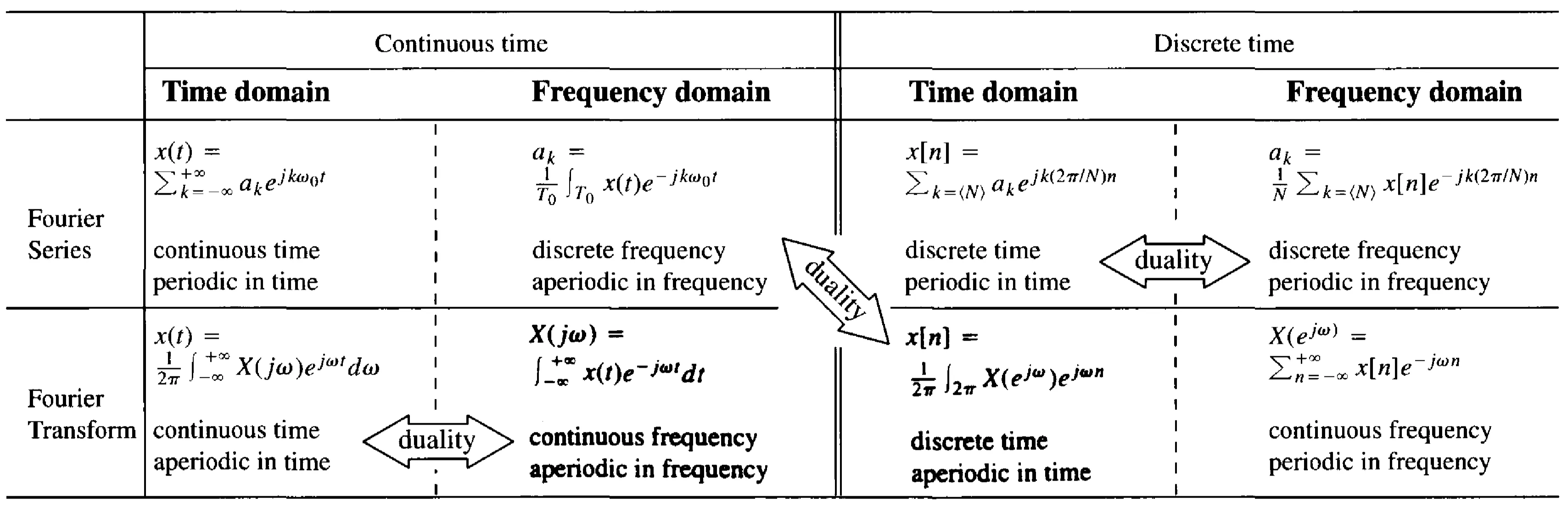
5.4 Duality

A notable duality exists that interrelates the mathematical forms of different Fourier representations. Specifically, there is a strong structural similarity between the Discrete-Time Fourier Transform (DTFT) and the Continuous-Time Fourier Series (CTFS).
The DTFT analysis equation is $X (e^{i ω}) = \sum_{n = - \infty}^{\infty} x [n] e^{- i ω n}$ . This involves a summation over a discrete variable $n$ and produces a continuous, periodic function of $ω$ .
The CTFS synthesis equation is $x (t) = \sum_{k = - \infty}^{\infty} a_{k} e^{i k ω_{0} t}$ . This involves a summation over a discrete variable $k$ and produces a continuous, periodic function of $t$ .
A similar structural correspondence exists between the DTFT synthesis equation (integral over continuous $ω$ to get discrete $x [n]$ ) and the CTFS analysis equation (integral over continuous $t$ to get discrete $a_{k}$ ). By appropriately interchanging time and frequency variables, and summation with integration, these transform pairs exhibit a formal duality.

Attachments/Oppenheim,Willsky_Signals and Systems 24.webp|700