Jump back to chapter selection.

Table of Contents

4.1 Representation of Aperiodic Signals: The Continuous-Time Fourier Transform
4.2 Convergence of Fourier Transforms
4.3 Properties of the Continuous-Time Fourier Transform
4.4 Basic Fourier Transform Pairs
4.5 Systems Characterised by Linear Constant-Coefficient Differential Equations

4 Continuous-Time Fourier Transform

A large class of signals, including all signals with finite energy, can be represented as a linear combination (or more generally, an integral) of complex exponentials. For periodic signals, as discussed in Chapter 3, these complex exponential building blocks are harmonically related, leading to a discrete sum in the Fourier series representation. For aperiodic signals, the constituent frequencies are infinitesimally close, and the representation takes the form of an integral rather than a sum. The resulting continuous spectrum of complex amplitudes is called the Fourier transform, and the synthesis integral used to reconstruct the signal from its spectrum is called the inverse Fourier transform.

The Fourier transform was one of Joseph Fourier's most significant contributions. He developed the intuition that an aperiodic signal could be viewed as a periodic signal in the limit where its period $T$ approaches infinity. As the period increases ( $T \to \infty$ ), the fundamental frequency $ω_{0} = 2 π / T$ decreases ( $ω_{0} \to 0$ ), and the harmonically related components $k ω_{0}$ become infinitesimally close in frequency. In this limit, the Fourier series sum transitions into an integral.

4.1 Representation of Aperiodic Signals: The Continuous-Time Fourier Transform

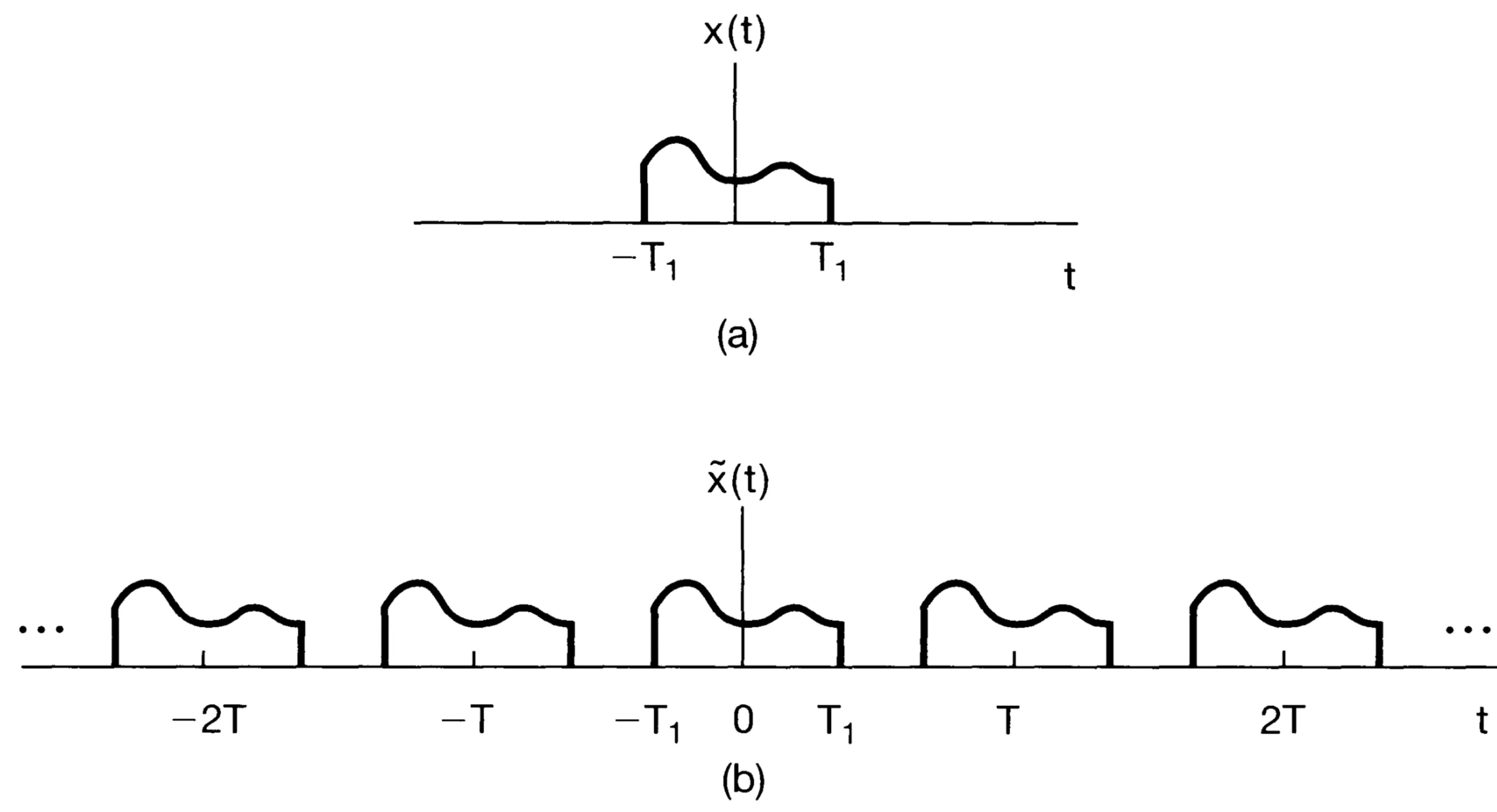
4.1.1 Example: From Periodic Square Wave to Aperiodic Rectangular Pulse

Consider a periodic square wave $x_{T} (t)$ with period $T$ , defined over one period as:

x_{T} (t) = {\begin{cases} 1, & for | t | < T_{1}, \\ 0, & for T_{1} < | t | \leq T / 2, \end{cases}

where $2 T_{1} < T$ . The Fourier series coefficients $a_{k}$ for this periodic signal are given by:

a_{k} = \frac{1}{T} \int_{- T_{1}}^{T_{1}} 1 \cdot e^{- i k ω_{0} t} d t = \frac{2 \sin (k ω_{0} T_{1})}{k ω_{0} T} = \frac{2 T_{1}}{T} sinc (\frac{k ω_{0} T_{1}}{π}),

where $ω_{0} = 2 π / T$ and $sinc (x) = \sin (π x) / (π x)$ . The quantity $T a_{k} = \frac{2 \sin (k ω_{0} T_{1})}{k ω_{0}}$ represents the samples of an envelope function.
As $T \to \infty$ , the periodic square wave $\tilde{x} (t)$ approaches a single, aperiodic rectangular pulse $x (t)$ (equal to 1 for $| t | < T_{1}$ and 0 otherwise). In this limit, $ω_{0} \to 0$ , and $k ω_{0}$ becomes a continuous variable $ω$ . The values $T a_{k}$ become samples of a continuous function (the envelope) $X (i ω) = \frac{2 \sin (ω T_{1})}{ω}$ . This envelope is the Fourier transform of the rectangular pulse.

4.1.2 Derivation

For a general aperiodic signal $x (t)$ (assumed to be of finite duration for this heuristic derivation, or otherwise satisfying convergence conditions), we can construct a periodic signal $\tilde{x} (t)$ by repeating $x (t)$ with a period $T$ , such that $x (t)$ is one period of $\tilde{x} (t)$ .

Attachments/Oppenheim,Willsky_Signals and Systems 19.webp|700

As $T \to \infty$ , $\tilde{x} (t)$ becomes identical to $x (t)$ for all $t$ . The Fourier series representation of $\tilde{x} (t)$ is:

\tilde{x} (t) = \sum_{k = - \infty}^{\infty} a_{k} e^{i k ω_{0} t}, with a_{k} = \frac{1}{T} \int_{- T / 2}^{T / 2} \tilde{x} (t) e^{- i k ω_{0} t} d t,

where $ω_{0} = 2 π / T$ . Since $\tilde{x} (t) = x (t)$ for $- T / 2 \leq t < T / 2$ (and $x (t) = 0$ outside this range if we consider $x (t)$ as the single period), then $a_{k} = \frac{1}{T} \int_{- \infty}^{\infty} x (t) e^{- i k ω_{0} t} d t$ .
Let us define the envelope $X (i ω)$ of $T a_{k}$ as $ω \to k ω_{0}$ :

X (i ω) = lim_{T \to \infty} (T a_{k}) = lim_{T \to \infty} \int_{- T / 2}^{T / 2} x (t) e^{- i (k ω_{0}) t} d t = \int_{- \infty}^{\infty} x (t) e^{- i ω t} d t .

Now, substitute $a_{k} = \frac{1}{T} X (i k ω_{0}) = \frac{ω_{0}}{2 π} X (i k ω_{0})$ into the Fourier series for $\tilde{x} (t)$ :

\tilde{x} (t) = \sum_{k = - \infty}^{\infty} (\frac{ω_{0}}{2 π} X (i k ω_{0})) e^{i k ω_{0} t} = \frac{1}{2 π} \sum_{k = - \infty}^{\infty} X (i k ω_{0}) e^{i k ω_{0} t} ω_{0} .

As $T \to \infty$ , $ω_{0} = Δ ω \to d ω$ , and the summation becomes an integral (a Riemann sum definition):

x (t) = \frac{1}{2 π} \int_{- \infty}^{\infty} X (i ω) e^{i ω t} d ω .

Thus, the continuous-time Fourier transform (CTFT) pair is:

Analysis (Forward FT): X (i ω) = \int_{- \infty}^{\infty} x (t) e^{- i ω t} d t

Synthesis (Inverse FT): x (t) = \frac{1}{2 π} \int_{- \infty}^{\infty} X (i ω) e^{i ω t} d ω

Here, $X (i ω)$ is called the Fourier transform, spectrum, or spectral density of $x (t)$ . It represents the complex amplitude of the constituent exponential $e^{i ω t}$ in $x (t)$ .

4.2 Convergence of Fourier Transforms

Although the heuristic derivation assumed $x (t)$ has finite duration, the CTFT pair applies to a broader class of signals, including many of infinite duration. The existence and convergence of the Fourier transform integral $X (i ω)$ and the inverse transform integral (reconstructing $x (t)$ ) depend on the properties of $x (t)$ . Let $\hat{x} (t)$ be the signal reconstructed by the inverse transform:

\hat{x} (t) = \frac{1}{2 π} \int_{- \infty}^{\infty} X (i ω) e^{i ω t} d ω .

Sufficient conditions for the Fourier transform $X (i ω)$ to exist and for $\hat{x} (t)$ to represent $x (t)$ include:

$x (t)$ is square integrable (i.e., $x (t)$ has finite energy): $\int_{- \infty}^{\infty} | x (t) |^{2} d t < \infty .$ If this condition holds, then $X (i ω)$ also has finite energy ( $\int_{- \infty}^{\infty} | X (i ω) |^{2} d ω < \infty$ , by Parseval's relation), and the inverse transform converges to $x (t)$ in the mean-square sense. That is, the energy of the difference $e (t) = \hat{x} (t) - x (t)$ is zero.
$x (t)$ satisfies the Dirichlet conditions:
- $x (t)$ is absolutely integrable: $\int_{- \infty}^{\infty} | x (t) | d t < \infty .$ (This condition alone guarantees that $X (i ω)$ is well-defined and bounded for all $ω$ ).
- $x (t)$ has a finite number of maxima and minima in any finite interval (bounded variation).
- $x (t)$ has a finite number of discontinuities in any finite interval, and each discontinuity must be finite.

If all three Dirichlet conditions are met, then $\hat{x} (t) = x (t)$ for all $t$ where $x (t)$ is continuous. At points of discontinuity, $\hat{x} (t)$ converges to the average of the values of $x (t)$ on either side of the discontinuity (the midpoint of the jump).

4.2.1 Periodic Signals and Impulses

Periodic signals, which are generally neither absolutely integrable nor square integrable over an infinite interval (they have infinite energy but finite power), can still have Fourier transforms if we permit the use of Dirac impulse functions in the frequency domain. For instance, the Fourier transform of $x (t) = e^{i ω_{0} t}$ is $X (i ω) = 2 π δ (ω - ω_{0})$ . This generalisation allows the Fourier series and Fourier transform to be unified within a common framework.

4.3 Properties of the Continuous-Time Fourier Transform

If $x (t) \overset{F T}{⟷} X (i ω)$ and $y (t) \overset{F T}{⟷} Y (i ω)$ , several useful properties hold:

Property	Aperiodic Signal $x (t), y (t)$	Fourier Transform $X (i ω), Y (i ω)$
Linearity	$a x (t) + b y (t)$	$a X (i ω) + b Y (i ω)$
Time Shifting	$x (t - t_{0})$	$e^{- i ω t_{0}} X (i ω)$
Frequency Shifting (Modulation)	$e^{i ω_{0} t} x (t)$	$X (i (ω - ω_{0}))$
Conjugation	$x^{*} (t)$	$X^{*} (- i ω)$
Time Reversal	$x (- t)$	$X (- i ω)$
Time and Frequency Scaling	$x (a t)$ , for real $a \neq 0$	$\frac{1}{a} X (\frac{i ω}{a})$
Convolution	$x (t) * y (t) = \int_{- \infty}^{\infty} x (τ) y (t - τ) d τ$	$X (i ω) Y (i ω)$
Multiplication	$x (t) y (t)$	$\frac{1}{2 π} (X (i ω) * Y (i ω)) = \frac{1}{2 π} \int_{- \infty}^{\infty} X (i θ) Y (i (ω - θ)) d θ$
Differentiation in Time	$\frac{d x (t)}{d t}$	$i ω X (i ω)$
Integration	$\int_{- \infty}^{t} x (τ) d τ$	$\frac{1}{i ω} X (i ω) + π X (0) δ (ω)$ (where $X (0) = \int x (t) d t$ )
Differentiation in Frequency	$t x (t)$	$i \frac{d X (i ω)}{d ω}$
Conjugate Symmetry for Real $x (t)$	$x (t)$ is real	$X (i ω) = X^{*} (- i ω)$ ; $Re [X (i ω)]$ is even, $Im [X (i ω)]$ is odd.
Symmetry for Real and Even $x (t)$	$x (t)$ is real and even	$X (i ω)$ is real and even.
Symmetry for Real and Odd $x (t)$	$x (t)$ is real and odd	$X (i ω)$ is purely imaginary and odd.
Even-Odd Decomp. for Real $x (t)$	$x_{e} (t) = E v {x (t)}$ , $x_{o} (t) = O d {x (t)}$	$x_{e} (t) \leftrightarrow Re [X (i ω)]$ ; $x_{o} (t) \leftrightarrow i Im [X (i ω)]$
Parseval's Relation	$\int_{- \infty}^{\infty} x (t)^{2} d t$	$\frac{1}{2 π} \int_{- \infty}^{\infty} X (i ω)^{2} d ω$

Parseval's Relation

If $x (t)$ and $X (i ω)$ are a Fourier transform pair (using $i ω$ or $j ω$ interchangeably for notation), then Parseval's relation states:

\int_{- \infty}^{+ \infty} | x (t) |^{2} d t = \frac{1}{2 π} \int_{- \infty}^{+ \infty} | X (i ω) |^{2} d ω .

This relation can be derived by starting with the integral of $| x (t) |^{2}$ :

\begin{aligned} \int_{- \infty}^{+ \infty} | x (t) |^{2} d t & = \int_{- \infty}^{+ \infty} x (t) x^{*} (t) d t . \end{aligned}

Substitute the inverse Fourier transform for $x^{*} (t)$ : $x^{*} (t) = {(\frac{1}{2 π} \int_{- \infty}^{\infty} X (i ω^{'}) e^{i ω^{'} t} d ω^{'})}^{*} = \frac{1}{2 π} \int_{- \infty}^{\infty} X^{*} (i ω^{'}) e^{- i ω^{'} t} d ω^{'}$ .

\begin{aligned} \int_{- \infty}^{+ \infty} | x (t) |^{2} d t & = \int_{- \infty}^{+ \infty} x (t) [\frac{1}{2 π} \int_{- \infty}^{+ \infty} X^{*} (i ω^{'}) e^{- i ω^{'} t} d ω^{'}] d t . \end{aligned}

Reversing the order of integration (assuming conditions allow):

\int_{- \infty}^{+ \infty} | x (t) |^{2} d t = \frac{1}{2 π} \int_{- \infty}^{+ \infty} X^{*} (i ω^{'}) [\int_{- \infty}^{+ \infty} x (t) e^{- i ω^{'} t} d t] d ω^{'} .

The bracketed term is the Fourier transform $X (i ω^{'})$ . Thus:

\int_{- \infty}^{+ \infty} | x (t) |^{2} d t = \frac{1}{2 π} \int_{- \infty}^{+ \infty} X^{*} (i ω^{'}) X (i ω^{'}) d ω^{'} = \frac{1}{2 π} \int_{- \infty}^{+ \infty} | X (i ω^{'}) |^{2} d ω^{'} .

The term on the left-hand side, $\int_{- \infty}^{\infty} | x (t) |^{2} d t$ , is the total energy in the signal $x (t)$ (if $x (t)$ represents a voltage or current across a 1-ohm resistor, for instance). Parseval's relation states that this total energy can be determined either by integrating the energy per unit time ( $| x (t) |^{2}$ ) over all time, or by integrating the energy per unit angular frequency ( $| X (i ω) |^{2} / (2 π)$ ) over all frequencies. For this reason, $| X (i ω) |^{2}$ is often referred to as the energy-density spectrum of the signal $x (t)$ . This relation for finite-energy aperiodic signals is the direct counterpart to Parseval's relation for periodic signals, which relates the average power of a periodic signal to the sum of the powers of its harmonic components.

4.4 Basic Fourier Transform Pairs

Signal $x (t)$	Fourier Transform $X (i ω)$	Fourier Series Coefficients $a_{k}$ (if $x (t)$ is periodic with period $T = 2 π / ω_{0}$ )
$\sum_{k = - \infty}^{\infty} a_{k} e^{i k ω_{0} t}$	$2 π \sum_{k = - \infty}^{\infty} a_{k} δ (ω - k ω_{0})$	$a_{k}$
$e^{i ω_{0} t}$	$2 π δ (ω - ω_{0})$	$a_{1} = 1$ (if $ω_{0}$ is fundamental), $a_{k} = 0$ for $k ω_{0} \neq ω_{0}$
$\cos (ω_{0} t)$	$π [δ (ω - ω_{0}) + δ (ω + ω_{0})]$	$a_{1} = a_{- 1} = 1 / 2$ , $a_{k} = 0$ for $k \neq 1$
$\sin (ω_{0} t)$	$\frac{π}{i} [δ (ω - ω_{0}) - δ (ω + ω_{0})]$	$a_{1} = 1 / (2 i), a_{- 1} = - 1 / (2 i)$ , $a_{k} = 0$ for $k \neq 1$
$1$ (DC signal)	$2 π δ (ω)$	$a_{0} = 1$ , $a_{k} = 0$ for $k \neq 0$
Rectangular pulse: $x (t) = 1$ for $t < T_{1}$ , $0$ else	$\frac{2 \sin (ω T_{1})}{ω} = 2 T_{1} sinc (\frac{ω T_{1}}{π})$	Not periodic
$δ (t)$ (unit impulse)	$1$	Not periodic
$u (t)$ (unit step)	$\frac{1}{i ω} + π δ (ω)$	Not periodic
$δ (t - t_{0})$	$e^{- i ω t_{0}}$	Not periodic
$e^{- a t} u (t)$ , $Re [a] > 0$	$\frac{1}{a + i ω}$	Not periodic
$t e^{- a t} u (t)$ , $Re [a] > 0$	$\frac{1}{(a + i ω)^{2}}$	Not periodic
Gaussian: $e^{- a t^{2}}$ , $a > 0$	$\sqrt{\frac{π}{a}} e^{- ω^{2} / (4 a)}$	Not periodic

Note: The specific Fourier Series coefficients for periodic signals depend on the choice of fundamental period $T = 2 π / ω_{0}$ . The sinc function used for the rectangular pulse is $sinc (x) = \sin (π x) / (π x)$ .

4.5 Systems Characterised by Linear Constant-Coefficient Differential Equations

Continuous-time LTI systems are often described by linear constant-coefficient differential equations of the general form:

\sum_{k = 0}^{N} a_{k} \frac{d^{k} y (t)}{d t^{k}} = \sum_{k = 0}^{M} b_{k} \frac{d^{k} x (t)}{d t^{k}} .

The frequency response $H (i ω)$ of such a system can be found by applying the Fourier transform to both sides of the equation. Using the differentiation property $F {\frac{d^{k} f (t)}{d t^{k}}} = (i ω)^{k} F (i ω)$ , we obtain:

\sum_{k = 0}^{N} a_{k} (i ω)^{k} Y (i ω) = \sum_{k = 0}^{M} b_{k} (i ω)^{k} X (i ω) .

The frequency response $H (i ω) = Y (i ω) / X (i ω)$ is therefore:

H (i ω) = \frac{\sum_{k = 0}^{M} b_{k} (i ω)^{k}}{\sum_{k = 0}^{N} a_{k} (i ω)^{k}} .

Thus, for systems described by linear constant-coefficient differential equations, the frequency response $H (i ω)$ is a rational function of $i ω$ (a ratio of polynomials in $i ω$ ).