Jump back to chapter selection.

Table of Contents

3.1 The Response of LTI Systems to Complex Exponentials
3.2 Fourier Series Representation of Continuous-Time Periodic Signals
3.3 Convergence of the Fourier Series
3.4 Properties of the Continuous-Time Fourier Series
3.5 Fourier Series Representation of Discrete-Time Periodic Signals
3.6 Properties of the Discrete-Time Fourier Series
3.7 Fourier Series and LTI Systems
3.8 Filtering
3.9 Important Examples: Continuous-Time
3.10 Important Examples: Discrete-Time Filters

3 Fourier Series Representation of Periodic Signals

The representation and analysis of LTI systems through the convolution sum, as discussed in Chapter 2, are based on representing signals as linear combinations of shifted impulses. This chapter explores an alternative and powerful representation for periodic signals and for the analysis of LTI systems, known as the Fourier series.

3.1 The Response of LTI Systems to Complex Exponentials

In the study of LTI systems, it is particularly advantageous to represent signals as linear combinations of basic signals that possess two key properties:

The set of basic signals can be used to construct a broad and useful class of signals.
The response of an LTI system to each of these basic signals is simple in form, thus providing a convenient way to represent the system's response to any signal constructed as a linear combination of these basic signals.

Fourier analysis is highly significant because complex exponential signals satisfy these properties for LTI systems, in both continuous and discrete time. Specifically, the response of an LTI system to a complex exponential input is the same complex exponential, merely scaled by a complex amplitude factor:

\begin{aligned} Continuous time: & x (t) = e^{s t} ⟶ y (t) = H (s) e^{s t}, \\ Discrete time: & x [n] = z^{n} ⟶ y [n] = H (z) z^{n}, \end{aligned}

where $s$ (for continuous time) and $z$ (for discrete time) are complex numbers. The complex amplitude factor $H (s)$ or $H (z)$ is characteristic of the system and is called the system's transfer function or system function, evaluated at $s$ or $z$ . A signal $x$ for which the system output is $y = a \cdot x$ (where $a$ is a constant) is called an eigenfunction of the system, and the complex constant $a$ is the corresponding eigenvalue. Thus, complex exponentials are eigenfunctions of LTI systems.

3.1.1 Continuous-Time Proof

For a continuous-time LTI system with impulse response $h (t)$ , if the input is $x (t) = e^{s t}$ , the output $y (t)$ is given by the convolution integral:

y (t) = \int_{- \infty}^{\infty} h (τ) x (t - τ) d τ = \int_{- \infty}^{\infty} h (τ) e^{s (t - τ)} d τ .

We can rewrite this as:

y (t) = e^{s t} \int_{- \infty}^{\infty} h (τ) e^{- s τ} d τ .

If the integral converges, we define:

H (s) = \int_{- \infty}^{\infty} h (τ) e^{- s τ} d τ .

Then, the output is $y (t) = H (s) e^{s t}$ . Thus, $e^{s t}$ is an eigenfunction of the LTI system, and $H (s)$ (which is the Laplace transform of $h (t)$ ) is the corresponding eigenvalue.

3.1.2 Discrete-Time Proof

Similarly, for a discrete-time LTI system with impulse response $h [n]$ , if the input is $x [n] = z^{n}$ , where $z$ is a complex number, the output $y [n]$ is given by the convolution sum:

y [n] = \sum_{k = - \infty}^{\infty} h [k] x [n - k] = \sum_{k = - \infty}^{\infty} h [k] z^{n - k} .

Rewriting this:

y [n] = z^{n} \sum_{k = - \infty}^{\infty} h [k] z^{- k} .

If the sum converges, we define:

H (z) = \sum_{k = - \infty}^{\infty} h [k] z^{- k} .

Then, the output is $y [n] = H (z) z^{n}$ . Thus, $z^{n}$ is an eigenfunction of the discrete-time LTI system, and $H (z)$ (which is the Z-transform of $h [n]$ ) is the corresponding eigenvalue.

3.1.3 Decomposition of Signals

The eigenfunction property is powerful because if a general input signal can be decomposed into a linear combination of these eigenfunctions, then, by the superposition property of LTI systems, the output will be a linear combination of the corresponding scaled eigenfunctions. For instance, if a continuous-time input $x (t)$ can be written as:

x (t) = \sum_{k} a_{k} e^{s_{k} t},

then the output of an LTI system with transfer function $H (s)$ is:

y (t) = \sum_{k} a_{k} H (s_{k}) e^{s_{k} t} .

A similar relationship holds for discrete-time signals represented as a sum of $z_{k}^{n}$ . This forms the basis of Fourier analysis, where periodic signals are decomposed into harmonically related complex exponentials $e^{i k ω_{0} t}$ (a special case of $e^{s t}$ with $s = i k ω_{0}$ ).

3.2 Fourier Series Representation of Continuous-Time Periodic Signals

A continuous-time periodic signal $x (t)$ with fundamental period $T$ (and fundamental frequency $ω_{0} = 2 π / T$ ) can often be represented as a linear combination of harmonically related complex exponentials:

x (t) = \sum_{k = - \infty}^{\infty} a_{k} e^{i k ω_{0} t} = \sum_{k = - \infty}^{\infty} a_{k} e^{i k (2 π / T) t} .

This is the complex exponential Fourier series representation of $x (t)$ . The terms $e^{i k ω_{0} t}$ are the harmonic components, and $a_{k}$ are the Fourier series coefficients.

3.2.1 Real Signals

If $x (t)$ is a real-valued signal, its Fourier series coefficients must satisfy the conjugate symmetry condition: $a_{k}^{*} = a_{- k}$ . This allows the series to be written in alternative forms. Using $a_{0}$ (the DC component) and pairing terms for $k$ and $- k$ :

x (t) = a_{0} + \sum_{k = 1}^{\infty} (a_{k} e^{i k ω_{0} t} + a_{- k} e^{- i k ω_{0} t}) = a_{0} + \sum_{k = 1}^{\infty} (a_{k} e^{i k ω_{0} t} + a_{k}^{*} e^{- i k ω_{0} t}) .

If we write $a_{k} = A_{k} e^{i θ_{k}}$ for $k \geq 1$ (where $A_{k} = | a_{k} |$ and $θ_{k} = \arg [a_{k}]$ ), and $a_{0}$ is real if $x (t)$ is real, then:

x (t) = a_{0} + \sum_{k = 1}^{\infty} 2 A_{k} \cos (k ω_{0} t + θ_{k}) .

Alternatively, using $a_{k} = B_{k} + i C_{k}$ (for $k \geq 1$ , $B_{k} = Re [a_{k}], C_{k} = Im [a_{k}]$ ), and noting $a_{0}$ is real:

x (t) = a_{0} + 2 \sum_{k = 1}^{\infty} (B_{k} \cos (k ω_{0} t) - C_{k} \sin (k ω_{0} t)) .

3.2.2 Derivation of Fourier Coefficients

Assuming $x (t)$ has a Fourier series representation as given above, we can determine the coefficients $a_{k}$ . Multiply both sides of the synthesis equation by $e^{- i n ω_{0} t}$ (where $n$ is an integer) and integrate over one period $T$ (from any $t_{0}$ to $t_{0} + T$ , commonly $0$ to $T$ or $- T / 2$ to $T / 2$ ):

\int_{T} x (t) e^{- i n ω_{0} t} d t = \int_{T} \sum_{k = - \infty}^{\infty} a_{k} e^{i k ω_{0} t} e^{- i n ω_{0} t} d t .

Interchanging the summation and integration (assuming convergence allows this):

\int_{T} x (t) e^{- i n ω_{0} t} d t = \sum_{k = - \infty}^{\infty} a_{k} \int_{T} e^{i (k - n) ω_{0} t} d t .

The integral on the right-hand side exploits the orthogonality of complex exponentials over one period:

\int_{T} e^{i (k - n) ω_{0} t} d t = {\begin{cases} T, & if k = n, \\ 0, & if k \neq n . \end{cases}

Thus, only the term where $k = n$ survives in the summation, yielding $T a_{n}$ . Relabelling $n$ as $k$ , the Fourier series coefficients are given by the analysis equation:

a_{k} = \frac{1}{T} \int_{T} x (t) e^{- i k ω_{0} t} d t .

The coefficient $a_{0}$ represents the average (DC) value of $x (t)$ over one period:

a_{0} = \frac{1}{T} \int_{T} x (t) d t .

3.3 Convergence of the Fourier Series

Although Joseph Fourier initially claimed that any periodic signal could be represented by a Fourier series, this is true only under certain conditions related to the "well-behavedness" of the signal.

3.3.1 Approximation and Error

The Fourier series represents $x (t)$ as an infinite sum. In practice, we often use a finite sum as an approximation:

x_{N} (t) = \sum_{k = - N}^{N} a_{k} e^{i k ω_{0} t} .

The approximation error is $e_{N} (t) = x (t) - x_{N} (t)$ . One measure of this error over one period is the integrated squared error (error energy per period):

E_{N} = \int_{T} | e_{N} (t) |^{2} d t .

It can be shown that the choice of coefficients $a_{k}$ given by the standard analysis formula minimises this mean square error $E_{N}$ . If $E_{N} \to 0$ as $N \to \infty$ , the series is said to converge in the mean-square sense.

3.3.2 Convergence Conditions (Dirichlet Conditions)

For a periodic signal $x (t)$ , its Fourier series representation (the infinite sum) converges to $x (t)$ (pointwise, except at discontinuities) if $x (t)$ satisfies the Dirichlet conditions over any one period:

$x (t)$ is absolutely integrable over one period: $\int_{T} | x (t) | d t < \infty$ . (This implies that $x (t)$ has finite energy over one period if it is also bounded, $\int_{T} | x (t) |^{2} d t < \infty$ , which is a condition for mean-square convergence).
$x (t)$ has a finite number of maxima and minima within any finite interval (bounded variation).
$x (t)$ has a finite number of discontinuities within any finite interval, and each discontinuity must be finite.

If these conditions are met, the Fourier series converges to $x (t)$ at all points where $x (t)$ is continuous. At points of discontinuity, the Fourier series converges to the average of the values of $x (t)$ on either side of the discontinuity (the midpoint of the jump).

3.3.3 Practical Implications

Most periodic signals encountered in engineering and physics satisfy the Dirichlet conditions and thus have Fourier series representations. Even if $x (t)$ and its Fourier series representation (the infinite sum) differ at a finite number of isolated points (specifically, at discontinuities), their integrals over any interval are identical, and their total energy or power per period are identical. For many practical purposes, particularly in the analysis of LTI systems, these isolated differences are not significant.

3.4 Properties of the Continuous-Time Fourier Series

If $x (t) \overset{F S}{⟷} a_{k}$ and $y (t) \overset{F S}{⟷} b_{k}$ (both periodic with period $T$ and fundamental frequency $ω_{0} = 2 π / T$ ), several useful properties hold:

Property	Periodic Signal $x (t), y (t)$	Fourier Series Coefficients $a_{k}, b_{k}$
Linearity	$A x (t) + B y (t)$	$A a_{k} + B b_{k}$
Time Shifting	$x (t - t_{0})$	$a_{k} e^{- i k ω_{0} t_{0}}$
Frequency Shifting	$e^{i M ω_{0} t} x (t)$ ( $M$ integer)	$a_{k - M}$
Conjugation	$x^{*} (t)$	$a_{- k}^{*}$
Time Reversal	$x (- t)$	$a_{- k}$
Time Scaling	$x (α t)$ ( $α > 0$ , new period $T / α$ )	$a_{k}$ (coefficients unchanged, fundamental frequency becomes $α ω_{0}$ )
Periodic Convolution	$\int_{T} x (τ) y (t - τ) d τ$	$T a_{k} b_{k}$
Multiplication	$x (t) y (t)$	$\sum_{l = - \infty}^{\infty} a_{l} b_{k - l}$ (discrete convolution)
Differentiation	$\frac{d x (t)}{d t}$	$i k ω_{0} a_{k}$
Integration	$\int_{- \infty}^{t} x (τ) d τ$ (periodic if $a_{0} = 0$ )	$\frac{1}{i k ω_{0}} a_{k}$ for $k \neq 0$ ; DC component needs separate consideration (may be non-zero if $a_{0} \neq 0$ for integral)
Conjugate Symmetry for Real $x (t)$	$x (t)$ is real	$a_{k} = a_{- k}^{*}$ ; $Re [a_{k}]$ is even, $Im [a_{k}]$ is odd; $a_{k}$ is even, $\arg [a_{k}]$ is odd.
For Real and Even $x (t)$	$x (t)$ is real and even	$a_{k}$ are real and even ( $a_{k} = a_{- k}$ )
For Real and Odd $x (t)$	$x (t)$ is real and odd	$a_{k}$ are purely imaginary and odd ( $a_{k} = - a_{- k}$ , $a_{0} = 0$ )
Even-Odd Decomp. of Real $x (t)$	$x_{e} (t) = \frac{x (t) + x (- t)}{2}$ , $x_{o} (t) = \frac{x (t) - x (- t)}{2}$	$x_{e} (t) \leftrightarrow Re [a_{k}]$ ; $x_{o} (t) \leftrightarrow i Im [a_{k}]$
Parseval's Relation	$\frac{1}{T} \int_{T} x (t)^{2} d t$	$\sum_{k = - \infty}^{\infty} a_{k}^{2}$

Note: For the Integration property, the indefinite integral is periodic only if $a_{0} = 0$ . If $a_{0} \neq 0$ , the integral contains a term $a_{0} t$ which is not periodic. The Fourier coefficient for $k = 0$ of the integral is generally undefined or needs special handling.

Parseval's Relation for Continuous-Time Periodic Signals

Parseval's relation for continuous-time periodic signals states that the average power of the signal is equal to the sum of the average powers of its individual harmonic components:

\frac{1}{T} \int_{T} | x (t) |^{2} d t = \sum_{k = - \infty}^{+ \infty} | a_{k} |^{2} .

The left-hand side is the average power of the periodic signal $x (t)$ over one period. The term $| a_{k} e^{i k ω_{0} t} |^{2} = | a_{k} |^{2}$ represents the power in the $k$ -th harmonic component (its average value over one period is $\frac{1}{T} \int_{T} | a_{k} |^{2} d t = | a_{k} |^{2}$ if we consider the power definition of $\frac{1}{T} \int | f (t) |^{2} d t$ for each component). Thus, Parseval's relation equates the total average power in a periodic signal to the sum of the average powers in all of its harmonic components.

3.5 Fourier Series Representation of Discrete-Time Periodic Signals

A discrete-time signal $x [n]$ is periodic with period $N$ if $x [n] = x [n + N]$ for all integers $n$ , where $N$ is a positive integer. The fundamental frequency is $ω_{0} = 2 π / N$ . The discrete-time Fourier series (DTFS) representation is a finite sum:

x [n] = \sum_{k = ⟨ N ⟩} a_{k} e^{i k ω_{0} n} = \sum_{k = 0}^{N - 1} a_{k} e^{i k (2 π / N) n},

where the sum can be taken over any $N$ consecutive integers $k$ . The Fourier series coefficients $a_{k}$ are given by:

a_{k} = \frac{1}{N} \sum_{n = ⟨ N ⟩} x [n] e^{- i k ω_{0} n} = \frac{1}{N} \sum_{n = 0}^{N - 1} x [n] e^{- i k (2 π / N) n} .

Both the signal $x [n]$ and its DTFS coefficients $a_{k}$ are periodic with period $N$ (i.e., $x [n + N] = x [n]$ and $a_{k + N} = a_{k}$ ). There are only $N$ distinct coefficients $a_{k}$ .

3.6 Properties of the Discrete-Time Fourier Series

If $x [n] \overset{D T F S}{⟷} a_{k}$ and $y [n] \overset{D T F S}{⟷} b_{k}$ (both periodic with period $N$ ), several useful properties hold (indices $k$ for $a_{k}, b_{k}$ are modulo $N$ ):

Property	Periodic Signal $x [n], y [n]$	Fourier Series Coefficients $a_{k}, b_{k}$
Linearity	$A x [n] + B y [n]$	$A a_{k} + B b_{k}$
Time Shifting	$x [n - n_{0}]$	$a_{k} e^{- i k ω_{0} n_{0}} = a_{k} e^{- i k (2 π / N) n_{0}}$
Frequency Shifting	$e^{i M ω_{0} n} x [n]$ ( $M$ integer)	$a_{k - M}$
Conjugation	$x^{*} [n]$	$a_{- k}^{*}$
Time Reversal	$x [- n]$	$a_{- k}$
Time Expansion (Upsampling)	$x_{(m)} [n] = {\begin{cases} x [n / m], & if n is a multiple of m \\ 0, & otherwise \end{cases}$ (Period $m N$ )	$b_{k} = \frac{1}{m} a_{k^{'}}$ where $k^{'} = k (\mod N)$ . The sequence $b_{k}$ has $m N$ unique values: $b_{k} = \frac{1}{m} a_{k}$ if $a_{k}$ repeated $m$ times. More precisely, $b_{k} = \frac{1}{m} a_{k}$ for original $a_{k}$ if spectrum viewed from $0$ to $m N - 1$ .
Periodic Convolution	$\sum_{r = ⟨ N ⟩} x [r] y [n - r]$	$N a_{k} b_{k}$
Multiplication	$x [n] y [n]$	$\sum_{l = ⟨ N ⟩} a_{l} b_{k - l}$ (circular convolution)
First Difference	$x [n] - x [n - 1]$	$(1 - e^{- i k ω_{0}}) a_{k}$
Running Sum	$y [n] = \sum_{m = - \infty}^{n} x [m]$ (periodic if $a_{0} = 0$ )	$b_{k} = \frac{1}{1 - e^{- i k ω_{0}}} a_{k}$ for $k ≢ 0 (\mod N)$ ; $b_{0}$ requires separate handling.
Conjugate Symmetry for Real $x [n]$	$x [n]$ is real	$a_{k} = a_{- k}^{*}$ ; $Re [a_{k}]$ is even, $Im [a_{k}]$ is odd (around $k = 0, N / 2$ ).
Parseval's Relation	$\frac{1}{N} \sum_{n = ⟨ N ⟩} x [n]^{2}$	$\sum_{k = ⟨ N ⟩} a_{k}^{2}$

Note for Time Expansion: If $x [n]$ has period $N$ and coefficients $a_{k}$ , the expanded signal $x_{(m)} [n]$ (with $m - 1$ zeros inserted between samples of $x [n]$ ) has period $m N$ . Its $m N$ DTFS coefficients $b_{k}$ are $b_{k} = (1 / m) a_{k / m}$ if $k$ is a multiple of $m$ , and $b_{k} = 0$ otherwise. Or, simply, the $N$ coefficients $a_{k}$ are scaled by $1 / m$ and "stretched" over $m N$ frequency bins by inserting zeros).

3.7 Fourier Series and LTI Systems

If a periodic signal $x (t)$ with Fourier series coefficients $a_{k}$ is input to an LTI system with frequency response $H (i ω)$ , the output $y (t)$ is also periodic with the same period and has Fourier series coefficients $b_{k}$ :

y (t) = \sum_{k = - \infty}^{\infty} a_{k} H (i k ω_{0}) e^{i k ω_{0} t} .

So, the Fourier coefficients of the output are $b_{k} = a_{k} H (i k ω_{0})$ . The system modifies the amplitude and phase of each harmonic component of the input. An analogous relationship holds for discrete-time LTI systems, where $b_{k} = a_{k} H (e^{i k ω_{0}})$ .

3.8 Filtering

Filtering is the process of modifying the amplitudes (and possibly phases) of the frequency components of a signal. An LTI system acts as a filter. Common types of filters include:

Low-pass filter (LPF): Passes low-frequency components (near $ω = 0$ ) and attenuates (reduces the amplitude of) higher-frequency components.
High-pass filter (HPF): Passes high-frequency components and attenuates lower-frequency components.
Bandpass filter (BPF): Passes frequency components within a specific band and attenuates components outside that band.

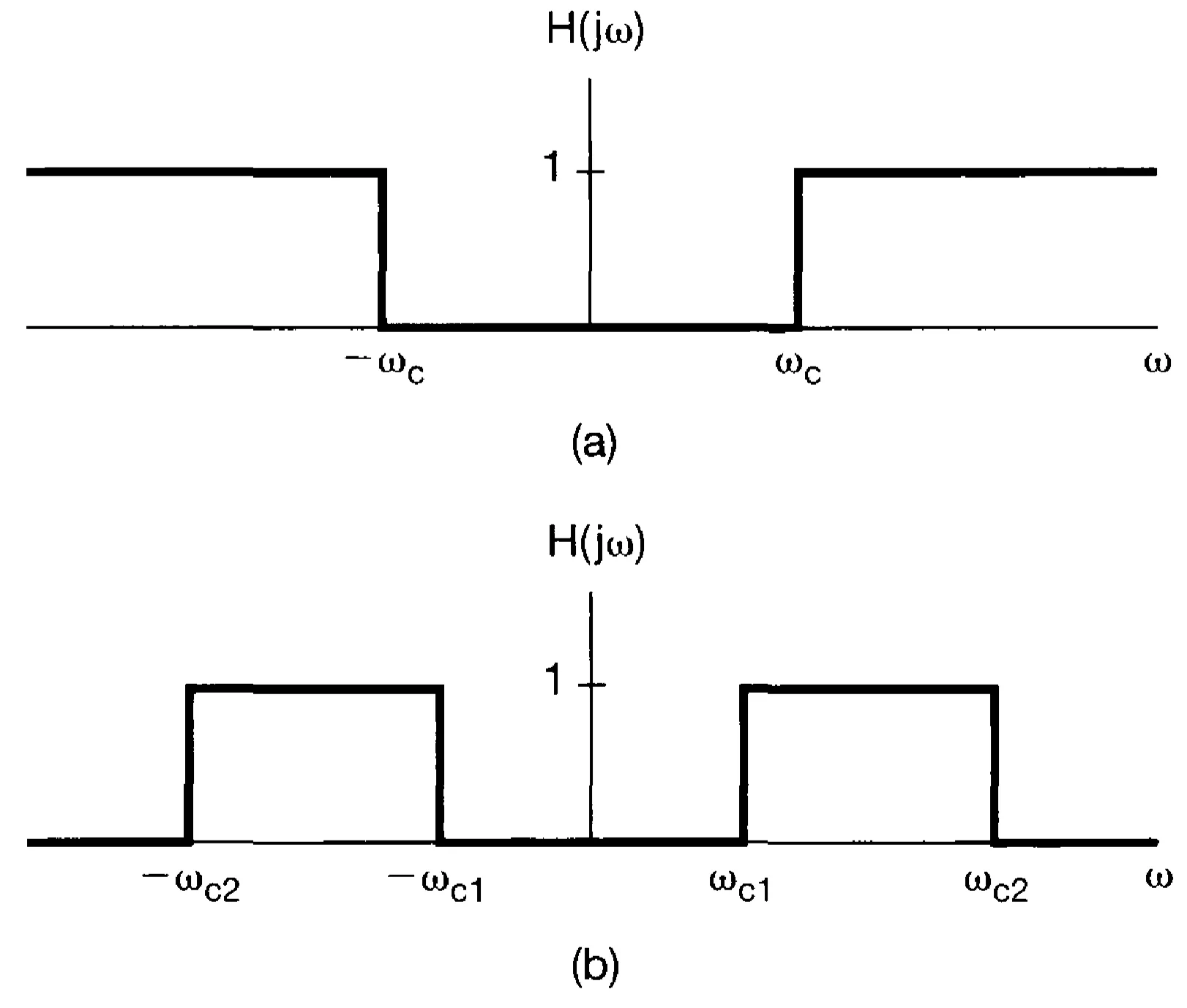
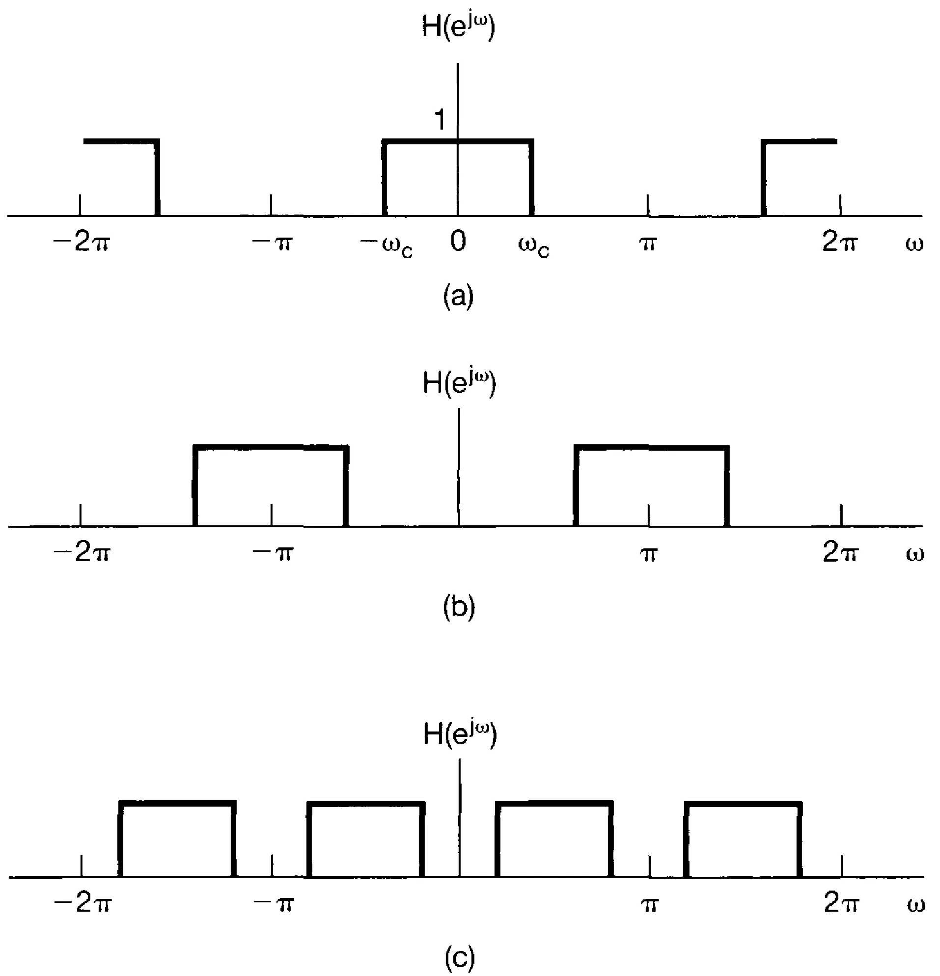
An ideal low-pass filter has a frequency response $H (i ω)$ that is constant (typically 1) within its passband and zero outside:

H_{ideal LPF} (i ω) = {\begin{cases} 1, & | ω | \leq ω_{c}, \\ 0, & | ω | > ω_{c}, \end{cases}

where $ω_{c}$ is the cutoff frequency. Ideal filters are not physically realisable but serve as useful conceptual models.
Ideal filters in continuous time and discrete time differ fundamentally because the frequency response $H (e^{i ω})$ of a discrete-time filter is always periodic in $ω$ with period $2 π$ , whereas $H (i ω)$ for a continuous-time filter is not necessarily periodic.

Visual examples of ideal filter frequency responses:

Continuous-time high-pass and bandpass filter:

Attachments/Oppenheim,Willsky_Signals and Systems 18.webp|700

Discrete-time low-pass, high-pass, and bandpass filter:

Attachments/Oppenheim,Willsky_Signals and Systems 17.webp|700

3.9 Important Examples: Continuous-Time

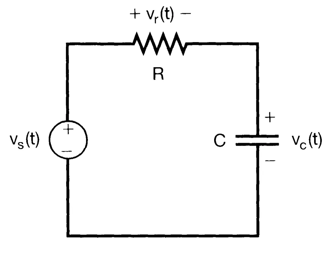
3.9.1 Simple RC Low-Pass Filter

Electrical circuits are commonly used to implement continuous-time filtering operations. One of the simplest examples is the first-order RC circuit shown below, where the input is $v_{s} (t)$ and the output is taken as the voltage across the capacitor, $v_{c} (t)$ .

Attachments/Oppenheim,Willsky_Signals and Systems 10.webp|700

The relationship between input and output is described by the linear constant-coefficient differential equation:

R C \frac{d v_{c} (t)}{d t} + v_{c} (t) = v_{s} (t) .

Assuming initial rest, this system is LTI. Its frequency response $H (i ω) = V_{c} (i ω) / V_{s} (i ω)$ can be found by taking the Fourier transform or by considering an input $v_{s} (t) = e^{i ω t}$ and finding the output $v_{c} (t) = H (i ω) e^{i ω t}$ :

H (i ω) = \frac{1}{1 + i ω R C} .

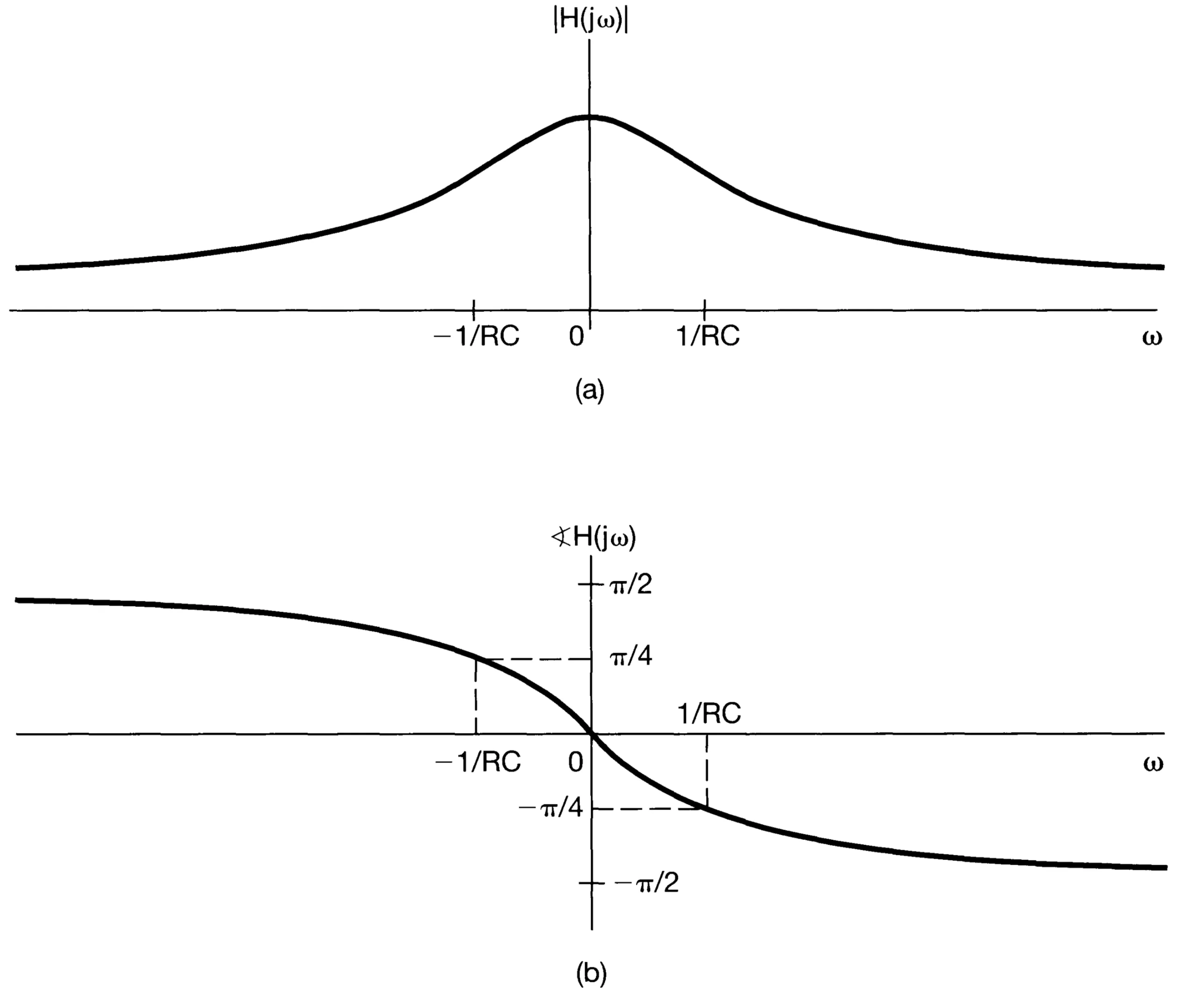
The magnitude and phase of $H (i ω)$ are plotted below:

Attachments/Oppenheim,Willsky_Signals and Systems 11.webp|700

For $ω \approx 0$ , $| H (i ω) | \approx 1$ , indicating that low frequencies pass with minimal attenuation. For higher $ω$ , $| H (i ω) |$ decreases (as $1 / (ω R C)$ for $ω R C ≫ 1$ ), making this circuit a non-ideal low-pass filter. The cutoff frequency ( $- 3 dB$ frequency) is $ω_{c} = 1 / (R C)$ .
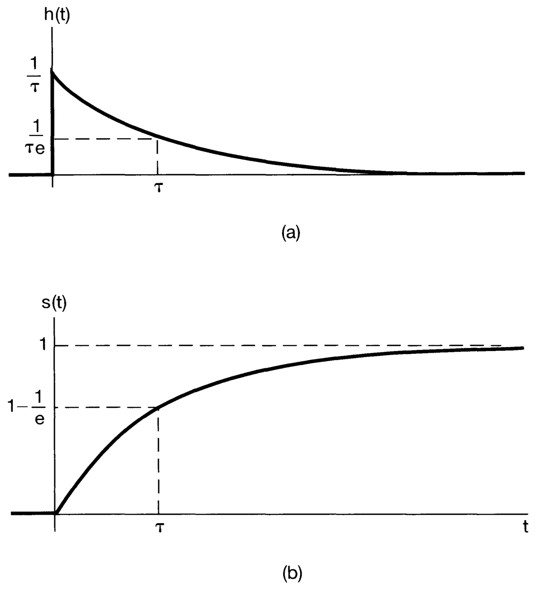
The impulse response and step response of the system are:

h (t) = \frac{1}{R C} e^{- t / (R C)} u (t),

s (t) = (1 - e^{- t / (R C)}) u (t) .

Attachments/Oppenheim,Willsky_Signals and Systems 12.webp|700

There is a trade-off between frequency-domain selectivity and time-domain behaviour. A larger $R C$ product (lower cutoff frequency) provides stronger low-pass filtering (attenuates high frequencies more) but results in a slower step response (longer rise time).

3.9.2 Simple RC High-Pass Filter

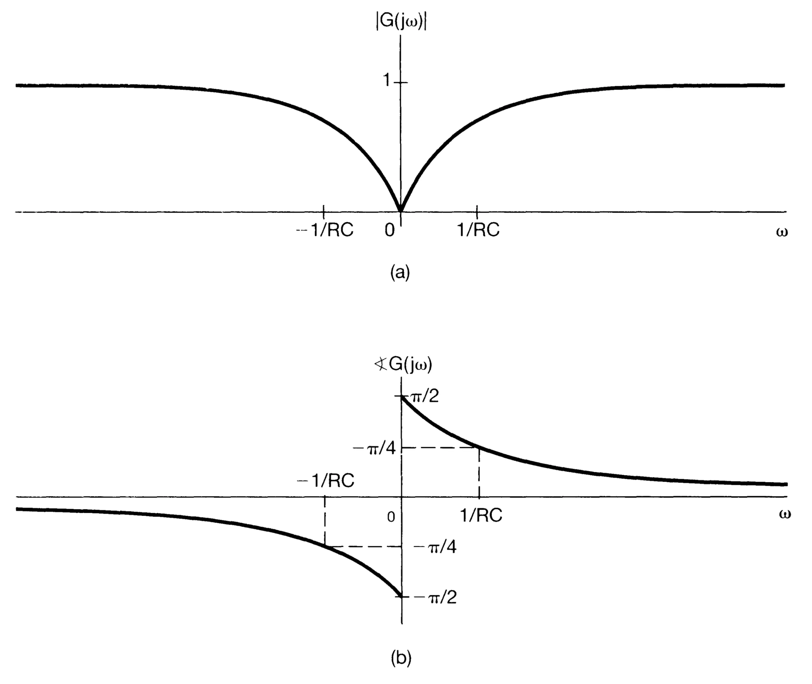
If we instead choose the resistor voltage $v_{r} (t)$ as the output in the same RC circuit, the system acts as a high-pass filter. The input-output relationship is $v_{s} (t) = v_{r} (t) + v_{c} (t)$ . Since $v_{r} (t) = R i (t)$ and $i (t) = C d v_{c} (t) / d t = C (d v_{s} (t) / d t - d v_{r} (t) / d t)$ , we get:

R C \frac{d v_{r} (t)}{d t} + v_{r} (t) = R C \frac{d v_{s} (t)}{d t} .

The frequency response $H_{H P} (i ω) = V_{r} (i ω) / V_{s} (i ω)$ is:

H_{H P} (i ω) = \frac{i ω R C}{1 + i ω R C} .

The magnitude and phase of $H_{H P} (i ω)$ are shown below:

Attachments/Oppenheim,Willsky_Signals and Systems 13.webp|700

This high-pass filter attenuates low frequencies (for $ω ≪ 1 / (R C)$ , $| H_{H P} (i ω) | \approx ω R C \to 0$ ) and allows high frequencies to pass (for $ω ≫ 1 / (R C)$ , $| H_{H P} (i ω) | \approx 1$ ).
As with the low-pass filter, increasing $R C$ shifts the cutoff frequency lower but also affects the transient response. More complex filter designs using additional energy storage elements (inductors, more capacitors) can achieve sharper transitions between passbands and stopbands and offer greater flexibility in shaping the frequency response.

3.10 Important Examples: Discrete-Time Filters

Discrete-time filters described by linear constant-coefficient difference equations are widely used in practice, particularly in digital signal processing. These filters are broadly categorised based on their impulse response duration:

Recursive filters (typically Infinite Impulse Response - IIR): The output depends on past output values as well as past and present input values. Their impulse responses generally have infinite length.
Non-recursive filters (typically Finite Impulse Response - FIR): The output depends only on past and present input values. Their impulse responses have finite length.

3.10.1 First-Order Recursive Discrete-Time Filters

A simple first-order recursive discrete-time filter is described by the difference equation:

y [n] - a y [n - 1] = x [n], or y [n] = a y [n - 1] + x [n] .

Assuming causality and initial rest, the frequency response $H (e^{i ω}) = Y (e^{i ω}) / X (e^{i ω})$ is:

H (e^{i ω}) = \frac{1}{1 - a e^{- i ω}} .

For stability, we require $| a | < 1$ .

For $0 < a < 1$ , the system acts as a low-pass filter (magnifies DC and low frequencies).
For $- 1 < a < 0$ , the system acts as a high-pass filter (magnifies high frequencies near $ω = π$ ).

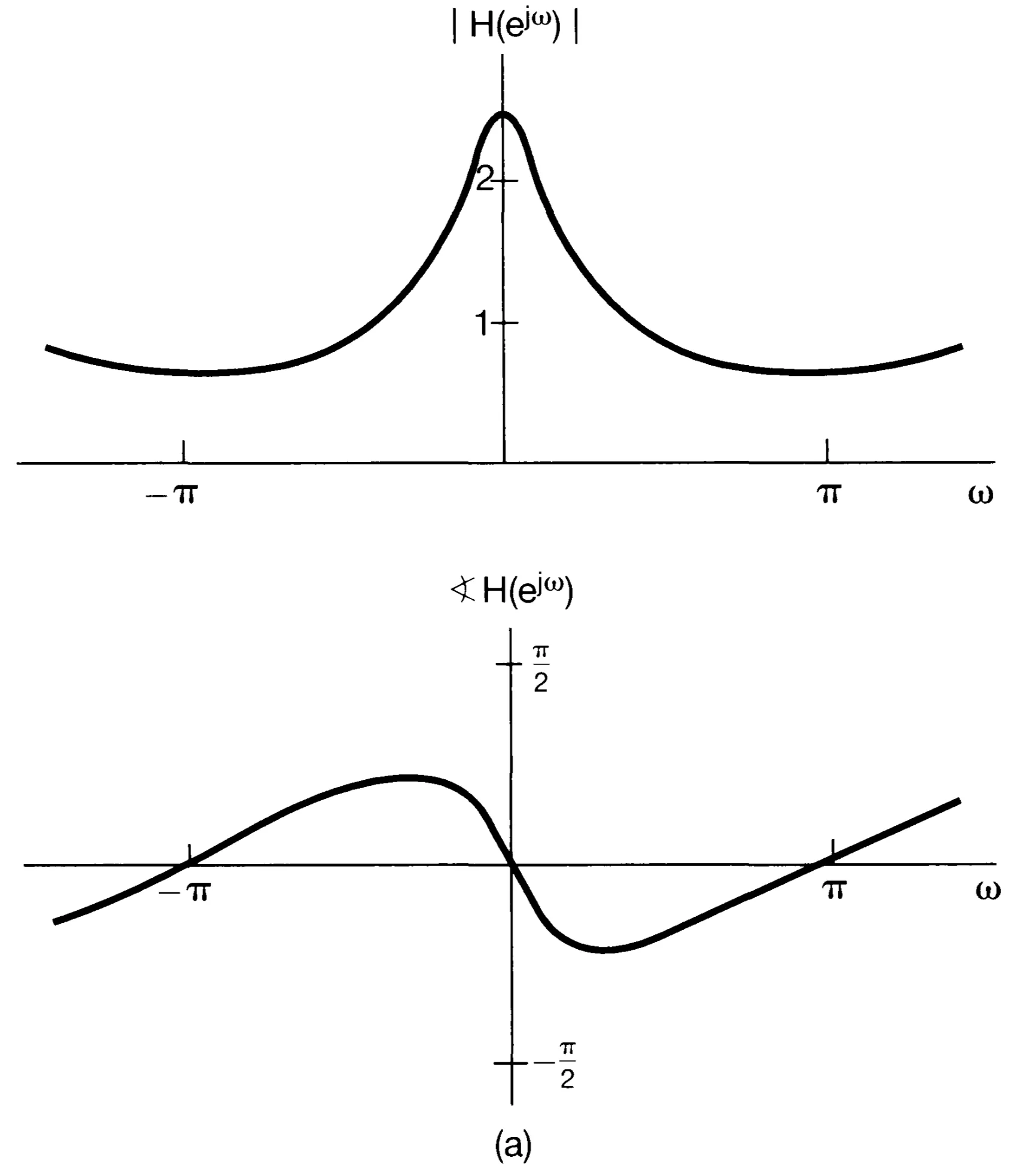
For $a = 0.6$ , the magnitude and phase of $H (e^{i ω})$ are shown below (low-pass characteristic):

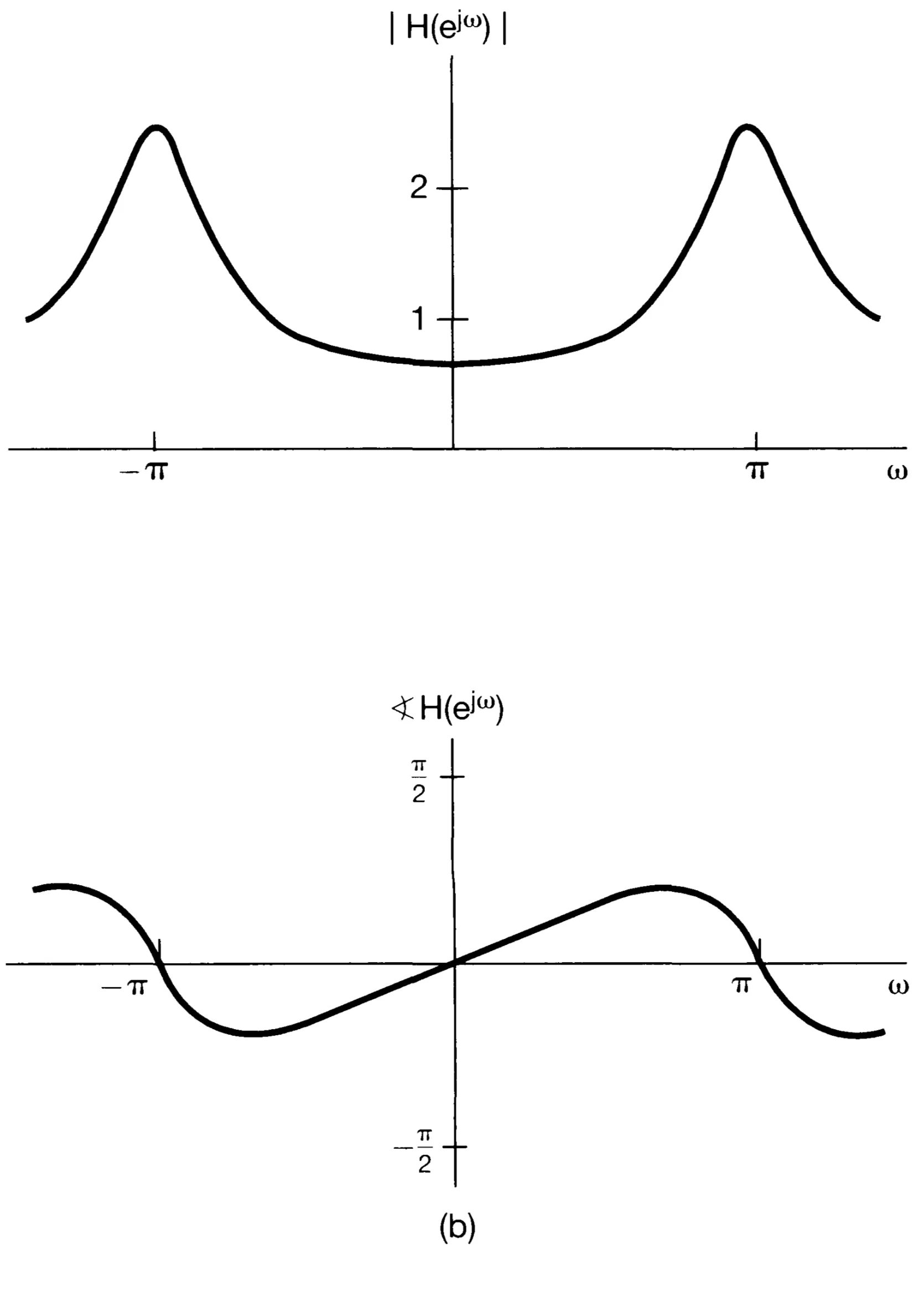
Attachments/Oppenheim,Willsky_Signals and Systems 14.webp|700

For $a = - 0.6$ , the magnitude and phase are as follows (high-pass characteristic):

Attachments/Oppenheim,Willsky_Signals and Systems 15.webp|700

The impulse response and step response are (for $| a | < 1$ ):

h [n] = a^{n} u [n],

s [n] = \sum_{k = 0}^{n} a^{k} u [n] = \frac{1 - a^{n + 1}}{1 - a} u [n] .

Higher-order recursive filters can provide sharper filtering characteristics and more complex frequency responses.

3.10.2 Non-Recursive Discrete-Time Filters

A general non-recursive (FIR) difference equation is:

y [n] = \sum_{k = M_{1}}^{M_{2}} b_{k} x [n - k] .

If $M_{1} < 0$ , the filter is non-causal. For a causal FIR filter, $M_{1} = 0$ , $y [n] = \sum_{k = 0}^{M} b_{k} x [n - k]$ .
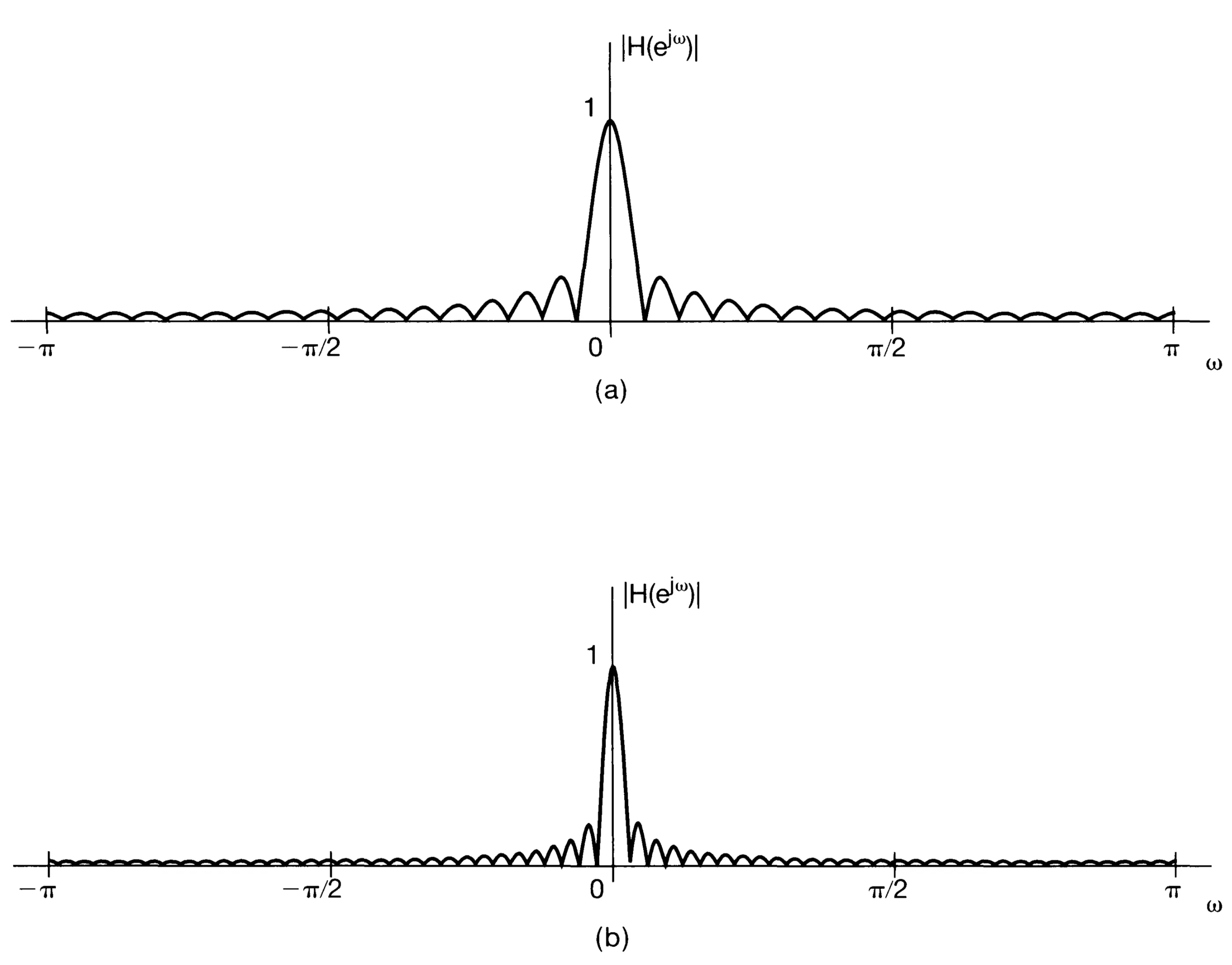
This equation represents a weighted average of $x [n]$ values. A common example is the moving-average filter, which typically uses uniform weights $b_{k} = 1 / (M_{2} - M_{1} + 1)$ . These filters smooth high-frequency variations in the input signal, effectively acting as low-pass filters.
For a causal moving-average filter of length $M + 1$ (sum from $k = 0$ to $M$ ) with weights $b_{k} = 1 / (M + 1)$ , the frequency response is:

H (e^{i ω}) = \frac{1}{M + 1} \sum_{k = 0}^{M} e^{- i k ω} = \frac{1}{M + 1} \frac{1 - e^{- i (M + 1) ω}}{1 - e^{- i ω}} = \frac{1}{M + 1} e^{- i M ω / 2} \frac{\sin ((M + 1) ω / 2)}{\sin (ω / 2)} .

The magnitude of $H (e^{i ω})$ for a causal moving average filter of length $L = 33$ and $L = 65$ (where $L = M + 1$ ) shows a main lobe at $ω = 0$ and sidelobes, with nulls at integer multiples of $2 π / L$ .

Attachments/Oppenheim,Willsky_Signals and Systems 16.webp|700