Jump back to chapter selection.

Table of Contents

2.1 The Convolution Sum
2.2 Convolution Properties of LTI Systems
2.3 Basic Properties
2.4 Causal LTI Systems Described by Differential Equations
2.5 Block Diagram Representation
2.6 Singularity Functions

2 Linear Time-Invariant Systems

In Chapter 1, a number of basic system properties were discussed. Two of these, linearity and time invariance, play a fundamental role in signal and system analysis for two major reasons. First, many physical processes possess these properties and thus can be modelled as linear time-invariant (LTI) systems. In addition, LTI systems can be analysed in considerable detail, providing both insight into their properties and a set of powerful tools that form the core of signal and system analysis.

One reason why LTI systems are of particular interest is that any such system possesses the superposition principle. As a consequence, if we can represent the input to an LTI system as a linear combination of a set of basic signals, we can then use superposition to compute the output of the system in terms of its responses to these basic signals. Unless stated otherwise, this chapter considers LTI systems.

2.1 The Convolution Sum

The so-called sifting property of the discrete-time unit impulse states that any discrete-time signal $x [n]$ can be represented as:

x [n] = \sum_{k = - \infty}^{\infty} x [k] δ [n - k] .

Because the sequence $δ [n - k]$ is non-zero (equal to 1) only when $k = n$ , the summation on the right-hand side effectively "sifts" through all the values in the sequence $x [k]$ and picks out (preserves) only the value $x [n]$ corresponding to the index $n$ . This property allows us to represent an arbitrary signal $x [n]$ as a superposition of scaled and shifted unit impulses.

Now, consider an LTI system. Let $h [n]$ be the response of this system to a unit impulse input $δ [n]$ (this is the definition of the impulse response).
Due to the time-invariance property, if $δ [n] \to h [n]$ , then a shifted input $δ [n - k]$ will produce a shifted output $h [n - k]$ .
Due to the linearity property (specifically, homogeneity and additivity), if the input is $x [n] = \sum_{k = - \infty}^{\infty} x [k] δ [n - k]$ , then the output $y [n]$ will be the sum of the responses to each scaled and shifted impulse:

y [n] = \sum_{k = - \infty}^{\infty} x [k] h [n - k] .

This operation is called the convolution sum or the superposition sum, and it is commonly denoted by an asterisk:

y [n] = x [n] * h [n] .

This is a fundamental result: an LTI system is completely characterised by its response to a single unit impulse, $h [n]$ . Knowing $h [n]$ allows us to calculate the output $y [n]$ for any input $x [n]$ using the convolution sum.

For continuous-time LTI systems, the same principles apply. The sifting property using the continuous-time unit impulse $δ (t)$ is:

x (t) = \int_{- \infty}^{\infty} x (τ) δ (t - τ) d τ .

If $h (t)$ is the impulse response of a continuous-time LTI system (i.e., the output when the input is $δ (t)$ ), then the output $y (t)$ for an arbitrary input $x (t)$ is given by the convolution integral (or superposition integral):

y (t) = x (t) * h (t) = \int_{- \infty}^{\infty} x (τ) h (t - τ) d τ .

2.2 Convolution Properties of LTI Systems

The convolution operation for LTI systems satisfies several important properties (shown here for continuous time, with analogous properties for discrete time):

Commutativity: The order of convolution does not matter. $x (t) * h (t) = h (t) * x (t)$
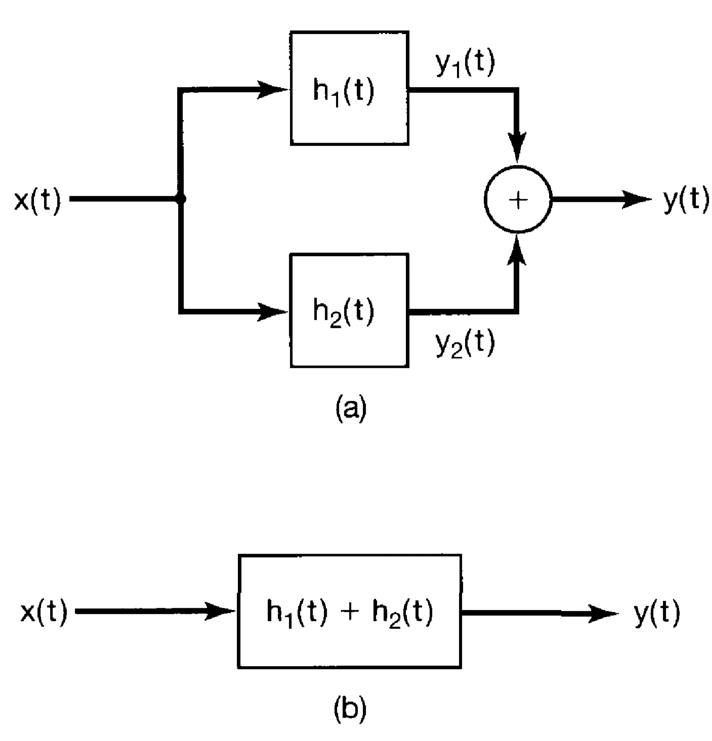
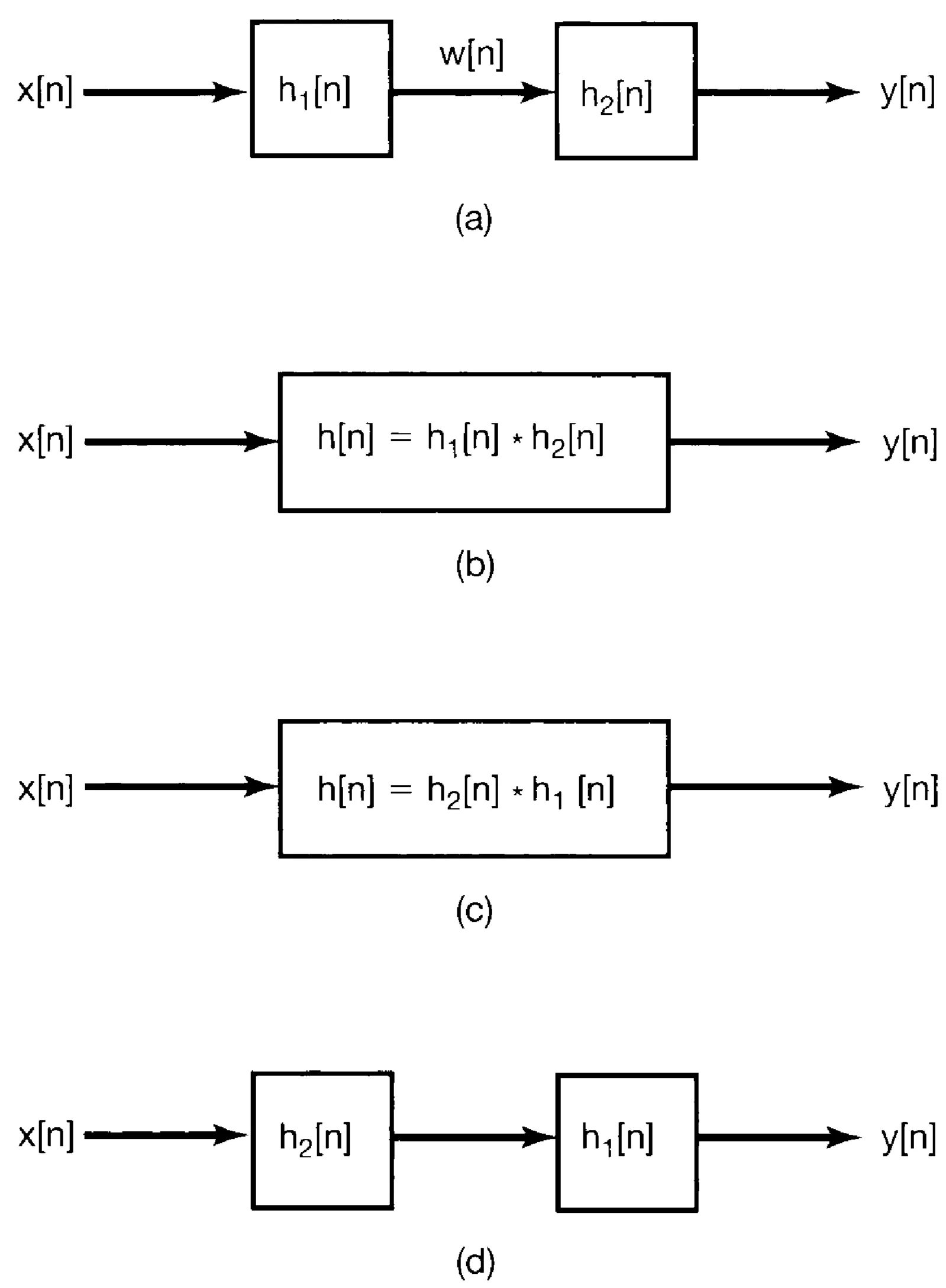
Distributivity: Convolution distributes over addition. This means a system with an impulse response $h_{1} (t) + h_{2} (t)$ (parallel combination) convolved with $x (t)$ is the same as $x (t)$ convolved with $h_{1} (t)$ plus $x (t)$ convolved with $h_{2} (t)$ . $x (t) * (h_{1} (t) + h_{2} (t)) = (x (t) * h_{1} (t)) + (x (t) * h_{2} (t))$
Associativity: The order of cascading LTI systems does not matter. $x (t) * (h_{1} (t) * h_{2} (t)) = (x (t) * h_{1} (t)) * h_{2} (t)$

Distributivity can be depicted graphically:

Attachments/Oppenheim,Willsky_Signals and Systems 5.webp|700

Similarly, associativity can be depicted graphically:

Attachments/Oppenheim,Willsky_Signals and Systems 6.webp|700

2.3 Basic Properties

The impulse response $h [n]$ or $h (t)$ of an LTI system provides complete information about the system and can be used to determine its other properties.

2.3.1 Memory

An LTI system is memoryless if its output depends only on the current input. This implies that its impulse response must be of the form $h [n] = K δ [n]$ for discrete-time systems, or $h (t) = K δ (t)$ for continuous-time systems, where $K$ is a constant. If $h [n]$ is non-zero for any $n \neq 0$ (or $h (t)$ is non-zero for $t \neq 0$ ), the system has memory.
If $K = 1$ , so $h (t) = δ (t)$ , then $y (t) = x (t) * δ (t) = x (t)$ . This is the identity system, and its impulse response is the unit impulse itself, consistent with the sifting property.

2.3.2 Invertibility

An LTI system with impulse response $h (t)$ is invertible if there exists an inverse system with impulse response $h_{inv} (t)$ such that when the two systems are cascaded, the overall output is equal to the original input. This means their combined impulse response is the unit impulse:

h (t) * h_{inv} (t) = δ (t) .

If an LTI system is invertible, its inverse is also an LTI system.

2.3.3 Causality

For an LTI system to be causal, its output $y (t)$ at any time $t_{0}$ must depend only on the input $x (t)$ for $t \leq t_{0}$ . This implies that the impulse response $h (t)$ must be zero for $t < 0$ (and $h [n] = 0$ for $n < 0$ in discrete time). The impulse response must be zero before the impulse occurs, which aligns with the intuitive concept of causality.
For linear systems (not necessarily time-invariant), causality is equivalent to the condition of initial rest: if the input $x (t) = 0$ for all $t < t_{0}$ , then the output $y (t) = 0$ must also be true for all $t < t_{0}$ .

2.3.4 Stability

An LTI system is Bounded-Input, Bounded-Output (BIBO) stable if and only if its impulse response is absolutely summable (for discrete time) or absolutely integrable (for continuous time):

\sum_{k = - \infty}^{\infty} | h [k] | < \infty (discrete time),

\int_{- \infty}^{\infty} | h (t) | d t < \infty (continuous time) .

If this condition holds, and if an input is bounded, $| x [n] | \leq B_{x} < \infty$ (or $| x (t) | \leq B_{x} < \infty$ ), then the output will also be bounded:

| y [n] | = | \sum_{k = - \infty}^{\infty} h [k] x [n - k] | \leq \sum_{k = - \infty}^{\infty} | h [k] | | x [n - k] | \leq B_{x} \sum_{k = - \infty}^{\infty} | h [k] | < \infty .

2.3.5 Unit Step Response of an LTI System

Besides the impulse response, another basic but important characterisation of an LTI system is its unit step response, $s (t)$ or $s [n]$ , which is the output when the input is the unit step function $u (t)$ or $u [n]$ .
For discrete time:

s [n] = u [n] * h [n] = \sum_{k = - \infty}^{n} h [k] .

For continuous time:

s (t) = u (t) * h (t) = \int_{- \infty}^{t} h (τ) d τ .

Conversely, the impulse response can be obtained from the step response:

h [n] = s [n] - s [n - 1], h (t) = \frac{d s (t)}{d t} .

2.4 Causal LTI Systems Described by Differential and Difference Equations

An important class of continuous-time LTI systems is those whose input $x (t)$ and output $y (t)$ are related by a linear constant-coefficient differential equation:

\sum_{k = 0}^{N} a_{k} \frac{d^{k} y (t)}{d t^{k}} = \sum_{k = 0}^{M} b_{k} \frac{d^{k} x (t)}{d t^{k}} .

These equations provide an implicit specification of the system. To obtain an explicit input-output expression (like the impulse response), one must solve the differential equation. The condition of initial rest (if the input is zero for $t < t_{0}$ , the output is zero for $t < t_{0}$ ) ensures that a system described by such an equation is linear, time-invariant, and causal.
For $N = 0$ (and $a_{0} \neq 0$ ), the system is memoryless if $M = 0$ , or involves differentiators if $M > 0$ .
For $N \geq 1$ , the solution $y (t)$ generally consists of two parts: a particular solution (forced response, dependent on the specific input $x (t)$ ) and a homogeneous solution (natural response, solution to the equation with $x (t) = 0$ ), which describes the system's intrinsic behaviour.

In discrete time, an analogous class of LTI systems is described by linear constant-coefficient difference equations:

\sum_{k = 0}^{N} a_{k} y [n - k] = \sum_{k = 0}^{M} b_{k} x [n - k] .

The natural response of this system satisfies $\sum_{k = 0}^{N} a_{k} y [n - k] = 0$ .
Assuming $a_{0} \neq 0$ , we can rewrite the difference equation to express $y [n]$ :

y [n] = \frac{1}{a_{0}} (\sum_{k = 0}^{M} b_{k} x [n - k] - \sum_{k = 1}^{N} a_{k} y [n - k]) .

If $N \geq 1$ , this equation is recursive because computing the current output $y [n]$ requires past output values $y [n - k]$ .

If $N = 0$ , the equation becomes $y [n] = \sum_{k = 0}^{M} \frac{b_{k}}{a_{0}} x [n - k]$ .
The impulse response is $h [n] = \frac{b_{n}}{a_{0}}$ for $0 \leq n \leq M$ , and $h [n] = 0$ otherwise. Such systems are non-recursive and have a Finite Impulse Response (FIR).
If $N \geq 1$ (recursive systems), the impulse response generally has infinite duration, and these systems are referred to as Infinite Impulse Response (IIR) systems.

2.5 Block Diagram Representation

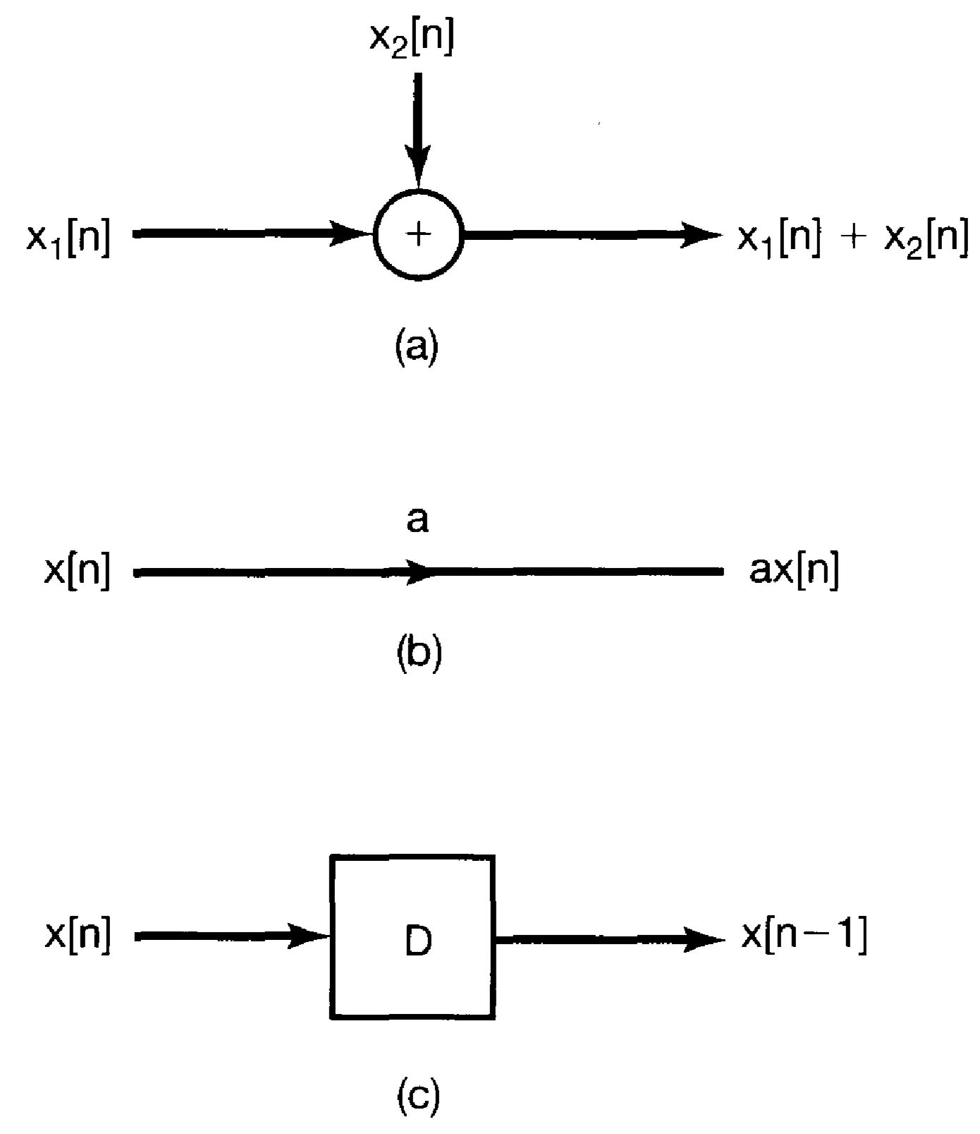
Systems described by linear constant-coefficient differential or difference equations can be represented using block diagrams. These diagrams provide a visual understanding of the system's structure and signal flow, and are valuable for both analysis and implementation. The basic elements are adders, multipliers (scalers), and delay elements (for discrete-time) or integrators (for continuous-time).

Consider the causal system described by the first-order difference equation (assuming $a_{0} = 1$ for simplicity, or normalising):

y [n] + a_{1} y [n - 1] = b_{0} x [n],

which can be rewritten as:

y [n] = b_{0} x [n] - a_{1} y [n - 1] .

This equation requires three basic operations: addition/subtraction, multiplication by a constant, and a unit delay:

Attachments/Oppenheim,Willsky_Signals and Systems 7.webp|700

The block diagram representation of this equation is:

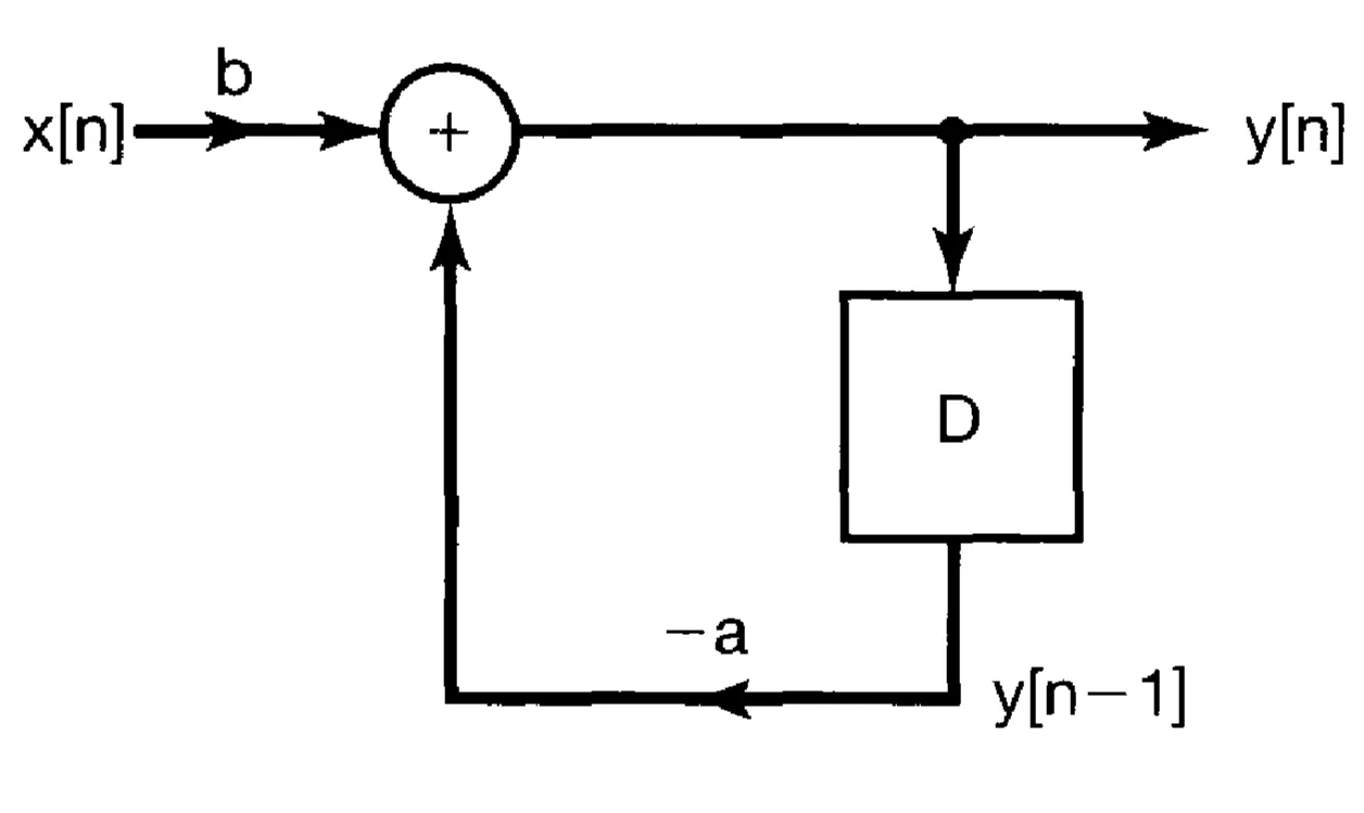
Attachments/Oppenheim,Willsky_Signals and Systems 8.webp|700

The feedback loop (output $y [n - 1]$ feeding back to compute $y [n]$ ) arises because the equation is recursive. The diagram clearly shows that memory (the delay element) is required for this system.

For a continuous-time system described by a first-order differential equation:

\frac{d y (t)}{d t} + a y (t) = b x (t) .

One way to implement this would be $y (t) = \frac{b}{a} x (t) - \frac{1}{a} \frac{d y (t)}{d t}$ (if $a \neq 0$ ). However, ideal differentiators are difficult to implement and are sensitive to noise. A more common approach is to use integrators by rewriting the equation as:

y (t) = \int_{- \infty}^{t} (b x (τ) - a y (τ)) d τ,

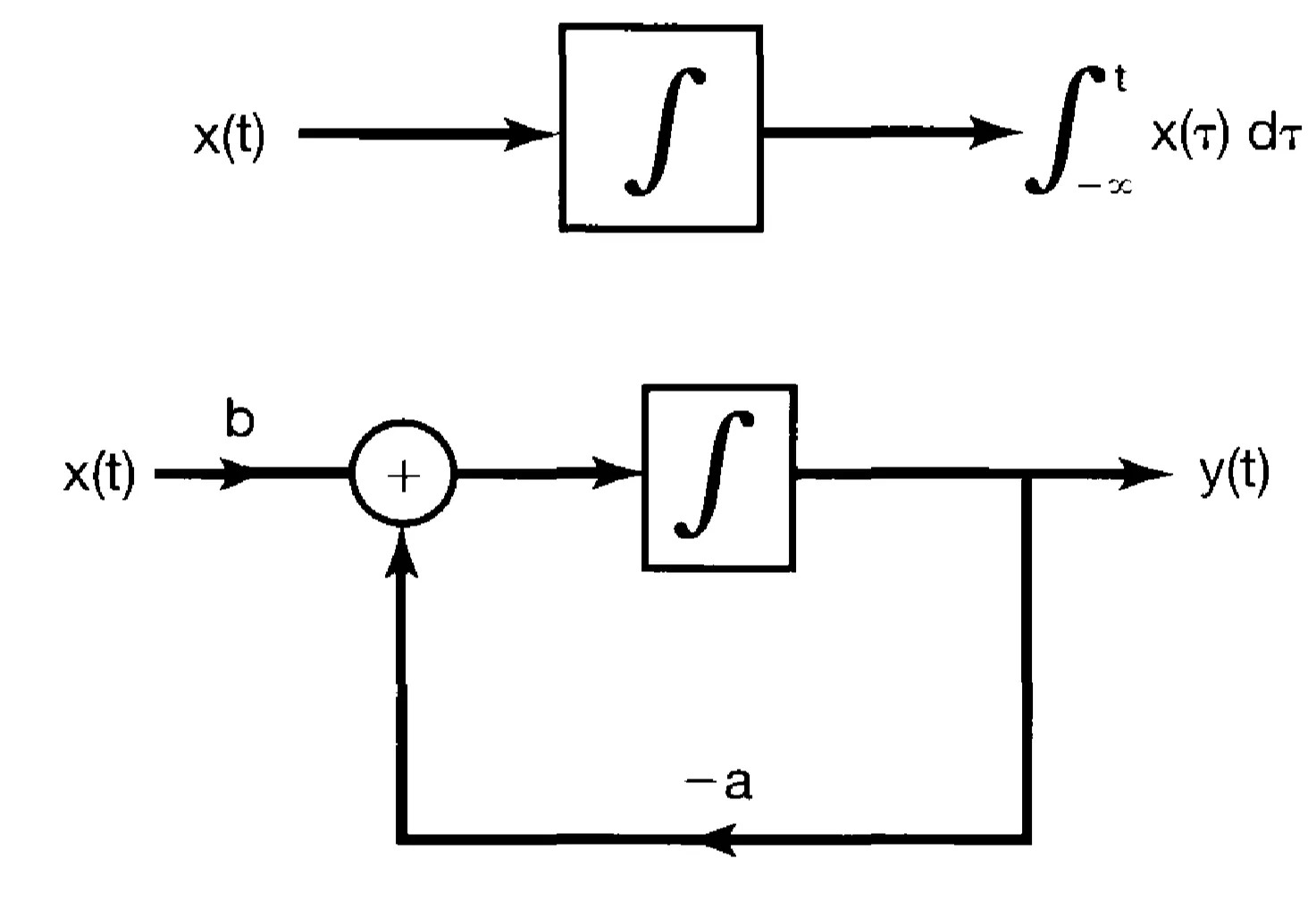
assuming $y (- \infty) = 0$ (initial rest). This can be implemented using integrators, adders, and scalers:

Attachments/Oppenheim,Willsky_Signals and Systems 9.webp|700

The integrator is inherently a memory element, as its output $y (t)$ depends on the past history of its input. This can also be seen from $y (t) = y (t_{0}) + \int_{t_{0}}^{t} (b x (τ) - a y (τ)) d τ$ , where the initial condition $y (t_{0})$ must be stored.

2.6 Singularity Functions

From the sifting property, the unit impulse $δ (t)$ is the impulse response of the identity system:

x (t) = x (t) * δ (t) .

Applying this to $δ (t)$ itself (letting $x (t) = δ (t)$ ):

δ (t) = δ (t) * δ (t) .

The unit impulse $δ (t)$ is an idealisation. It can be defined as the limit of a sequence of functions that become infinitely narrow and infinitely tall while maintaining unit area. Its crucial defining characteristic is its behaviour under convolution (the sifting property).
An equivalent operational definition, highlighting the sifting property, is that for any continuous function $g (t)$ :

\int_{- \infty}^{\infty} g (τ) δ (t - τ) d τ = g (t) and thus for t = 0, \int_{- \infty}^{\infty} g (τ) δ (τ) d τ = g (0) .

The unit impulse belongs to a class of signals known as singularity functions. A key property is:

f (t) δ (t - t_{0}) = f (t_{0}) δ (t - t_{0}),

assuming $f (t)$ is continuous at $t = t_{0}$ .

Higher-order singularity functions, such as the unit doublet $u_{1} (t)$ , unit triplet $u_{2} (t)$ , etc., are defined as successive derivatives of the unit impulse: $u_{k} (t) = \frac{d^{k} δ (t)}{d t^{k}} = δ^{(k)} (t)$ . Their convolution properties are:

x (t) * u_{k} (t) = \frac{d^{k} x (t)}{d t^{k}} .

For example, the response to a unit doublet $u_{1} (t) = δ^{'} (t)$ is $y (t) = x (t) * δ^{'} (t) = \frac{d x (t)}{d t}$ .

The unit step $u (t)$ is the integral of the unit impulse:

u (t) = \int_{- \infty}^{t} δ (τ) d τ (denoted as u_{- 1} (t) in some contexts) .

The unit ramp function $r (t) = t u (t)$ is the integral of the unit step:

r (t) = u_{- 2} (t) = \int_{- \infty}^{t} u (τ) d τ = u (t) * u (t) .

Higher-order integrals of $δ (t)$ (successive integrations of the unit step) can be generated by convolving $u (t)$ with itself:

u_{- k} (t) = \underset{k times}{\underset{⏟}{u (t) * \dots * u (t)}} = \int_{- \infty}^{t} u_{- (k - 1)} (τ) d τ .

This can be expressed in closed form as:

u_{- k} (t) = \frac{t^{k - 1}}{(k - 1)!} u (t) for k \geq 1.

The notation convention can be summarised: $u_{0} (t) = δ (t)$ , $u_{- 1} (t) = u (t)$ , and generally $u_{k} (t) = δ^{(k)} (t)$ for $k \geq 0$ , and $u_{k} (t)$ is the $(| k |)$ -th integral of $δ (t)$ for $k < 0$ .