Jump back to chapter selection.

Table of Contents

1.1 Continuous-Time and Discrete-Time Signals
1.2 Energy and Power
1.3 Transformations
1.4 Periodic Signals
1.5 Even and Odd Signals
1.6 Exponential Signals
1.7 Unit Impulse and Unit Step
1.8 Interconnection of Systems
1.9 Basic Properties

1 Signals and Systems

1.1 Continuous-Time and Discrete-Time Signals

Signals are represented mathematically as functions of one or more independent variables. Here, our attention is focused on signals involving a single independent variable, which we will usually denote as time $t$ for convenience. In the case of continuous-time signals, the independent variable is continuous, and thus these signals are defined for a continuum of values of the independent variable. On the other hand, discrete-time signals are defined only at discrete points in time; consequently, for these signals, the independent variable takes on only a discrete set of values.

For continuous-time signals, we will enclose the independent variable in parentheses, for instance $x(t)$. For discrete-time signals, we will use brackets to enclose the independent variable, for instance $x[n]$. A discrete-time signal $x[n]$ may represent a phenomenon for which the independent variable is inherently discrete. Demographic data, sampled at yearly intervals, is an example of this.

Alternatively, a very important class of discrete-time signals arises from the sampling of continuous-time signals. In this case, the discrete-time signal $x[n]$ represents successive samples of an underlying continuous phenomenon.

1.2 Energy and Power

In many applications, the signals considered are directly related to physical quantities such as power and energy in a physical system. As a starting example, consider a voltage $v(t)$ across a resistor with resistance $R$, causing a current $I(t)$ to flow. The instantaneous power dissipated in the resistor is $p(t)=v(t)I(t)=v^2(t)/R$. This allows us to calculate the total energy expended over the time interval $t_1\le t\le t_2$ as:

and the average power over this interval as:

With these simple physical examples in mind, it is conventional to use similar terminology for power and energy for any continuous-time signal $x(t)$ or any discrete-time signal $x[n]$, even if they do not directly represent physical power or energy. The "instantaneous power" is often taken to be proportional to $|x(t){|}^2$ or $|x[n]{|}^2$.

The total energy of a signal over a finite time interval $[t_1,t_2]$ (or $[n_1,n_2]$) is defined as:

The time-averaged power over this interval is:

For signals considered over an infinite time interval ($-\mathrm{\infty }<t<\mathrm{\infty }$ or $-\mathrm{\infty }<n<\mathrm{\infty }$), the total energy is:

Note that for some signals (for instance, a non-zero constant signal), this integral or sum might not converge, meaning such signals have infinite total energy. The time-averaged power over an infinite interval is then defined as:

These definitions allow us to identify three important classes of signals:

1. Finite total energy signals (Energy signals): These have $E_{\mathrm{\infty }}<\mathrm{\infty }$. For such signals, it follows that $P_{\mathrm{\infty }}=0$.
2. Finite average power signals (Power signals): These have $0<P_{\mathrm{\infty }}<\mathrm{\infty }$. For such signals, it follows that $E_{\mathrm{\infty }}=\mathrm{\infty }$. Periodic signals are a common example.
3. Signals with neither finite total energy nor finite average power, such as $x(t)=t$.

1.3 Transformations

A central concept in signal and system analysis is the transformation of an independent variable (usually time) of a signal. Such transformations are fundamental to understanding how signals are modified or how different signals relate to one another. Examples of systems performing signal transformations are abundant, including audio equalisers that modify the spectrum of a music signal or medical imaging systems that reconstruct an image from sensor data.

Some important and very fundamental transformations of the time variable are:

• Time shift: $x(t)\to x(t-t_0)$. This shifts the signal along the time axis by $t_0$. If $t_0>0$, the signal is delayed; if $t_0<0$, the signal is advanced.
• Time reversal (or reflection): $x(t)\to x(-t)$. This reflects the signal about the time origin $t=0$.
• Time scaling: $x(t)\to x(\alpha t)$. If $|\alpha |>1$, the signal is compressed in time. If $0<|\alpha |<1$, the signal is expanded in time. If $\alpha <0$, it also involves time reversal.

1.4 Periodic Signals

A very important class of signals encountered frequently is periodic signals. A continuous-time signal $x(t)$ is periodic if there exists a positive value $T$ such that:

In other words, a periodic signal is unchanged by a time shift of $T$. The signal $x(t)$ is then said to be periodic with period $T$. The fundamental period $T_0$ is defined as the smallest positive value of $T$ for which the periodicity condition holds. Any integer multiple of $T_0$, $m{T}_0$ (where $m$ is a positive integer), is also a period of $x(t)$.

1.5 Even and Odd Signals

Another set of useful properties of signals relates to their symmetry under time reversal. A signal $x(t)$ (or $x[n]$) is considered even if it is identical to its time-reversed counterpart:

A signal is considered odd if it is the negative of its time-reversed counterpart:

An odd signal must be zero at time zero (if defined at $t=0$ or $n=0$), since $x(-0)=-x(0)$ implies $x(0)=-x(0)$, so $2x(0)=0$, which means $x(0)=0$.
Any signal can be uniquely decomposed into a sum of an even part and an odd part:

where the even part $\mathcal{E}v\{x(t)\}$ and odd part $\mathcal{O}d\{x(t)\}$ are given by:

(Analogous definitions apply for discrete-time signals $x[n]$).

1.6 Exponential Signals

Consider the continuous-time complex exponential signal of the form $x(t)=C{e}^{\alpha t}$, where $C$ and $\alpha$ are, in general, complex numbers. Depending on the values of $C$ and $\alpha$, these signals can exhibit a variety of characteristics:

1. Real exponential signals: $C$ and $\alpha$ are real numbers.
   1. If $\alpha <0$, $x(t)$ represents an exponential decay.
   2. If $\alpha >0$, $x(t)$ represents an exponential growth.
   3. If $\alpha =0$, $x(t)=C$ is a constant (DC signal).
2. Periodic complex exponential signals (Purely imaginary $\alpha$ ): Let $\alpha =i{\omega }_0$, where ${\omega }_0$ is real. Then $x(t)=C{e}^{i{\omega }_{0}t}$. This signal is periodic with fundamental period $T_0=2\pi /|{\omega }_0|$ (if ${\omega }_0\ne 0$). If ${\omega }_0=0$, it is a DC signal, which is periodic with any period $T>0$. Like other non-zero periodic signals, these have infinite total energy but finite average power (specifically, $P_{\mathrm{\infty }}=|C{|}^2$).
3. General complex exponential signals: Let $C=|C|e^{i{\theta }_C}$ and $\alpha ={\sigma }_0+i{\omega }_0$. Then $x(t)=|C|e^{{\sigma }_{0}t}{e}^{i({\omega }_{0}t+{\theta }_C)}$.
   1. If $\mathfrak{Re}\left[\alpha \right]={\sigma }_0=0$: $x(t)$ is purely sinusoidal (as in point 2).
   2. If $\mathfrak{Re}\left[\alpha \right]={\sigma }_0>0$: $x(t)$ is a sinusoidal signal multiplied by an exponentially increasing envelope.
   3. If $\mathfrak{Re}\left[\alpha \right]={\sigma }_0<0$: $x(t)$ is a sinusoidal signal multiplied by an exponentially decaying envelope.

Many of the concepts discussed from section 1.3 to section 1.6 have direct analogues for discrete-time signals. However, a key difference arises in the periodicity of discrete-time complex exponentials: A discrete-time complex exponential $x[n]=e^{i{\omega }_{0}n}$ is periodic if and only if its frequency ${\omega }_0$ is a rational multiple of $2\pi$. That is, ${\omega }_0/(2\pi )=k/N$ for some integers $k$ and $N\ne 0$. This implies ${\omega }_{0}N=2\pi k$ must hold for some integer $N$, which is then a period.

1.7 Unit Impulse and Unit Step

In this section, several other basic signals of considerable importance in signal and system analysis are introduced.
Consider the discrete-time unit impulse (or unit sample), $\delta [n]$:

And the discrete-time unit step, $u[n]$:

There is a close relationship between the unit impulse and the unit step in discrete time. In particular, the unit impulse is the first difference of the unit step:

Conversely, the unit step is the running sum of the unit impulse:

An alternative form for the running sum (by change of variable $k=n-m$) is $u[n]=\sum _{k=0}^{\mathrm{\infty }}\delta [n-k]$.
A key property of the discrete-time unit impulse is the sifting property:

Summing over $n$ gives $\sum _{n}x[n]\delta [n-n_0]=x[n_0]$.

For continuous-time signals, the continuous-time unit impulse (or Dirac delta function) $\delta (t)$ and unit step $u(t)$ are analogous. The unit step is the integral of the unit impulse:

(This implies $u(t)=1$ for $t>0$ and $u(t)=0$ for $t<0$; the value at $t=0$ is often undefined or taken as $1/2$).
Conversely, the unit impulse is the derivative of the unit step:

The sifting property for the continuous-time impulse is ${\int }_{-\mathrm{\infty }}^{\mathrm{\infty }}x(t)\delta (t-t_0)dt=x(t_0)$.

The unit impulse should be considered an idealisation of a pulse that is infinitely short in duration, has unit area, and is infinitely tall. Any real physical system possesses some "inertia" or finite response time. The response of such a system to an input pulse that is sufficiently short (compared to the system's response time) is often independent of the exact pulse duration or shape, and depends primarily on its integrated effect (its area). For a system with a faster response, the input pulse must be shorter for this approximation to hold. The ideal unit impulse is considered short enough to probe the response of any linear time-invariant system.

1.8 Interconnection of Systems

An important concept in systems analysis is the interconnection of systems, since many real-world systems are constructed as interconnections of several simpler subsystems. By decomposing a complex system into an interconnection of simpler subsystems, it may be possible to analyse or synthesise it using basic building blocks. The most frequently encountered connections are the series (or cascade) and parallel types:

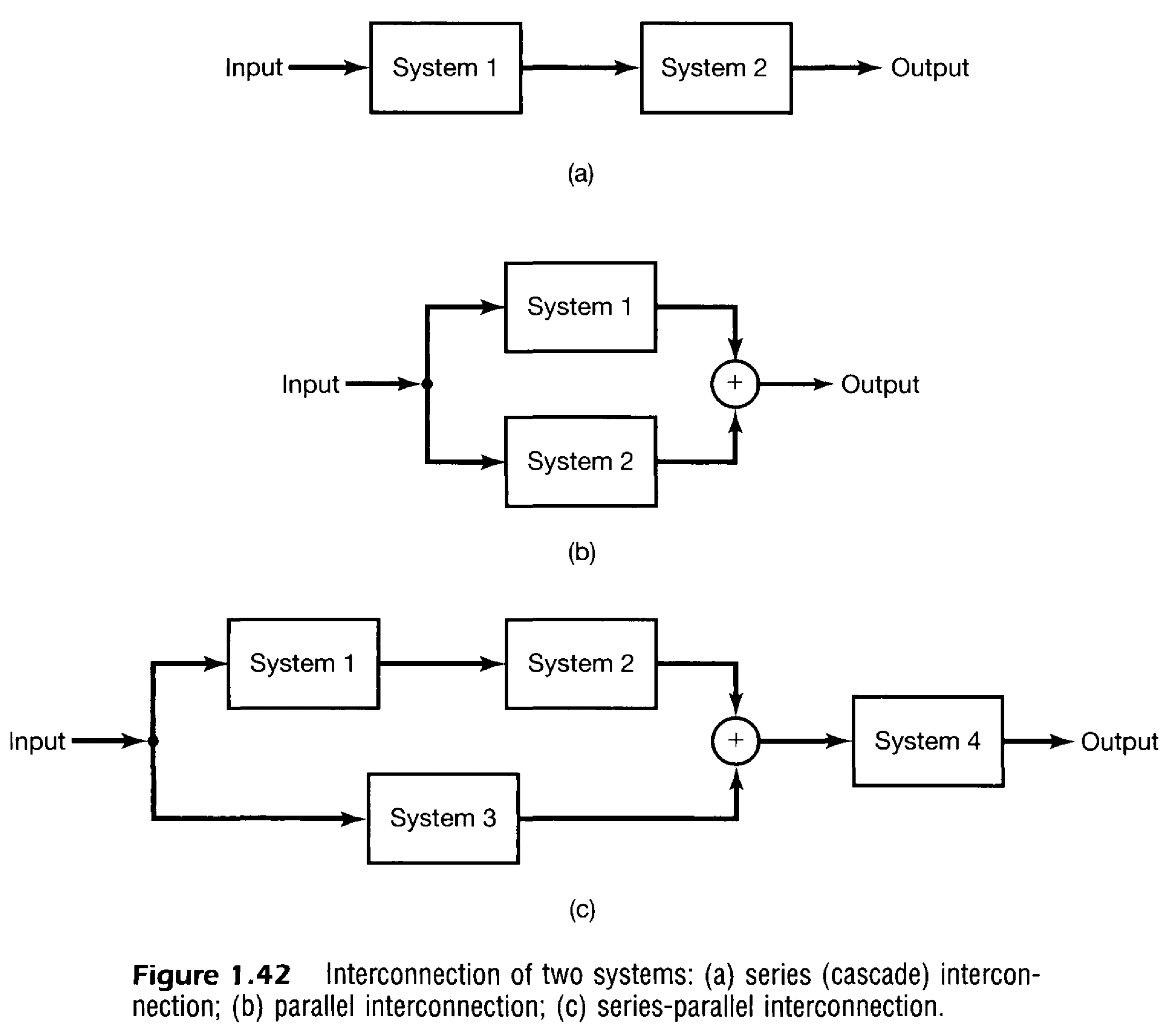
The symbol $⨁$ denotes addition of signals, so the output of the parallel system is the sum of the outputs from system 1 and system 2 (when both have the same input). Another important type of connection is the feedback interconnection:

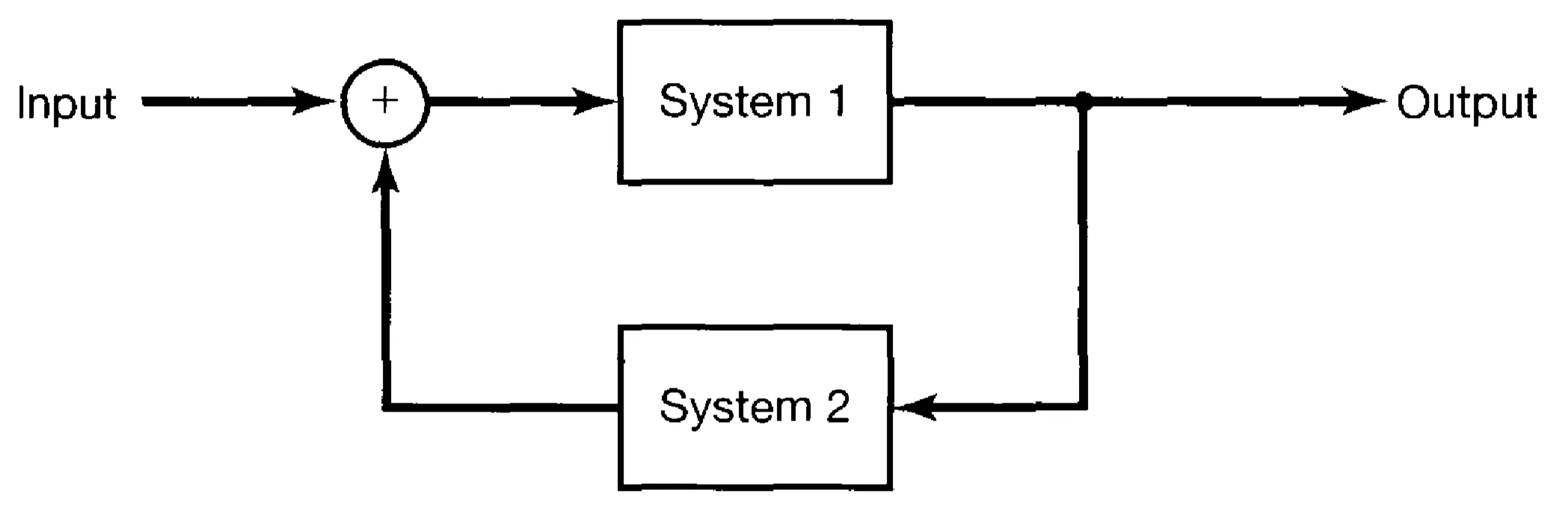
In this (negative) feedback configuration, the output of system 1 is the input to system 2. The output of system 2 is then fed back and subtracted from (or added to, for positive feedback) the external input to produce the actual input signal that drives system 1. These types of interconnections are prevalent in many practical systems, for instance, in control systems and amplifiers. Block diagram equivalences, such as shown below, are often useful for simplifying or analysing interconnected systems.

1.9 Basic Properties

1.9.1 Memory

A system is said to be memoryless if its output at any given time depends only on the input at that same time. An example of a basic memoryless system is the identity system, $y(t)=x(t)$ or $y[n]=x[n]$, where the output is simply equal to the input. Another is a resistor where $v(t)=Ri(t)$.

Systems that are not memoryless are said to possess memory. Their output depends on past (and for non-causal systems, possibly future) values of the input. As counterexamples:

• The accumulator system $y[n]=\sum _{k=-\mathrm{\infty }}^{n}x[k]$ has memory, as the output at time $n$ depends on all past and present inputs.
• The delay system $y[n]=x[n-1]$ also has memory, as the output at time $n$ depends on the input at time $n-1$.
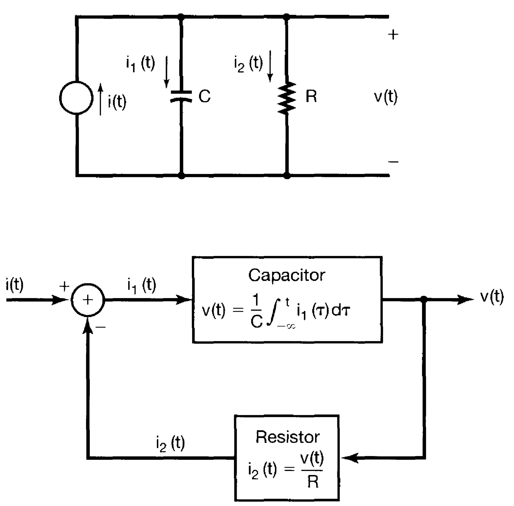
  A capacitor is an example of a physical system component with memory, since the voltage across it is $V(t)=\frac{1}{C}{\int }_{-\mathrm{\infty }}^{t}I(\tau )d\tau$, depending on the history of the current $I(\tau )$.

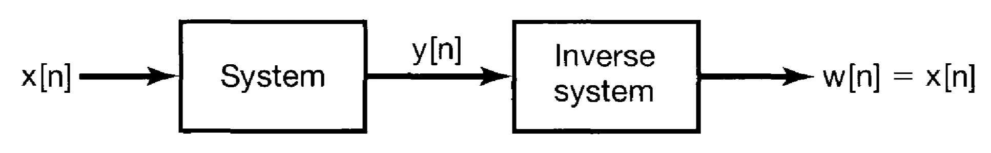
1.9.2 Invertibility and Inverse Systems

A system is said to be invertible if distinct inputs produce distinct outputs. If a system is invertible, then an inverse system exists which, when cascaded with the original system, yields an output equal to the original system's input. That is, if system $S$ produces $y(t)$ from $x(t)$, its inverse $S^{-1}$ produces $x(t)$ from $y(t)$.

Invertibility is important in many contexts, such as signal processing (for instance, deconvolution to remove distortions) and communication systems (for instance, decoding an encoded signal). Lossless data compression, for example, requires that the encoding process must be invertible to allow perfect reconstruction of the original data.

1.9.3 Causality

A system is causal if its output at any time $t$ (or $n$) depends only on values of the input at the present time and in the past (i.e., for $t^{\prime }\le t$ or $n^{\prime }\le n$). Such a system is also termed non-anticipative, as its output does not anticipate future values of the input. All real-time physical systems must be causal.
Examples of non-causal systems include:

1.9.4 Stability

A system is stable in the Bounded-Input, Bounded-Output (BIBO) sense if every bounded input signal produces an output signal that is also bounded. That is, if an input $x(t)$ satisfies $|x(t)|\le B_x<\mathrm{\infty }$ for all $t$ (where $B_x$ is a finite positive number), then the output $y(t)$ must satisfy $|y(t)|\le B_y<\mathrm{\infty }$ for all $t$ (where $B_y$ is also a finite positive number, which may depend on $B_x$).
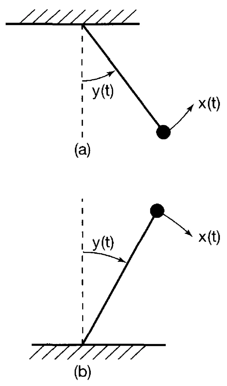
For instance, consider a simple pendulum with small oscillations (stable system) versus an inverted pendulum (unstable system): a small perturbation (input) to the inverted pendulum can lead to a large, unbounded output (falling over).

1.9.5 Time Invariance

A system is time-invariant if its behaviour and characteristics are fixed over time. Formally, a system is time-invariant if a time shift in the input signal causes an identical time shift in the output signal. That is, if an input $x[n]$ produces an output $y[n]$ (so $x[n]\to y[n]$), then for any arbitrary time shift $n_0$, the input $x_d[n]=x[n-n_0]$ must produce the output $y_d[n]=y[n-n_0]$. (An analogous definition applies for continuous-time systems with $t$ and $t_0$).

1.9.6 Linearity

A system is linear if it satisfies the superposition principle. This principle combines two properties:

1. Additivity: If input $x_1(t)$ produces output $y_1(t)$, and input $x_2(t)$ produces output $y_2(t)$, then the input $x_1(t)+x_2(t)$ must produce the output $y_1(t)+y_2(t)$.
2. Homogeneity (or Scaling): If input $x_1(t)$ produces output $y_1(t)$, then for any complex constant $\alpha$, the input $\alpha x_1(t)$ must produce the output $\alpha y_1(t)$.

These two properties can be combined into a single condition for superposition: for any inputs $x_1(t),x_2(t)$ and any complex constants $\alpha ,\beta$:

Analogous definitions apply for discrete-time systems.