Table of Contents

2.1 Single Mode Field Operators and Quadratures
2.2 Photon Number States
2.3 Coherent States
2.4 Squeezed Light

2 Quantum States of the Field

2.1 Single Mode Field Operators and Quadratures

We consider next a single-mode field, a single value of $k$ and a single polarisation index $σ$ . The single-mode electric field is

\hat{E} (χ) = E_{0} (\hat{a} e^{- i χ} + {\hat{a}}^{†} e^{i χ}) .

Introducing yet another set of operators, the quadrature operators ${\hat{a}}_{1}$ and ${\hat{a}}_{2}$ defined as

{\hat{a}}_{1} = \frac{\hat{a} + {\hat{a}}^{†}}{2}, {\hat{a}}_{2} = \frac{\hat{a} - {\hat{a}}^{†}}{2 i},

we can rewrite the electric field as

\hat{E} (χ) = \hat{X} \cos (χ) + \hat{Y} \sin (χ) .

It can then be shown that the commutation relation

[\hat{E} (χ_{1}), \hat{E} (χ_{2})] = - \frac{i}{2} {(2 E_{0})}^{2} \sin (χ_{1} - χ_{2})

holds. Remember this important relation between operators and commutator:

[\hat{A}, \hat{B}] = \hat{C} \Rightarrow Δ A \cdot Δ B \geq \frac{1}{2} | ⟨ \hat{C} ⟩ |

Applying this to the prior results yields the uncertainty in the field operator as

Δ \hat{E} (χ_{1}) Δ \hat{E} (χ_{2}) \geq \frac{1}{4} | \sin (χ_{1} - χ_{2}) | .

Note that in this expression, the field is measured in units of $2 E_{0}$ . What does this result imply? It means that we can measure 'exactly' single mode fields that differ by units of pi. However, we have the case where the difference is $χ_{1} - χ_{2} = π / 2$ , such that the uncertainty for the product of the field quadratures is

Δ \hat{X} \cdot Δ \hat{Y} \geq \frac{1}{4} {(2 E_{0})}^{2} .

2.2 Photon Number States

The photon number state is an eigenstate of the photon number operator $\hat{n} = {\hat{a}}^{†} \hat{a}$ . Therefore,

⟨ n | Δ \hat{n} | n ⟩ = 0 = ⟨ n | {\hat{n}}^{2} | n ⟩ - ⟨ n | \hat{n} | n ⟩^{2} .

Intuitively, it is a state where we have "perfect" knowledge of the intensity, but no knowledge of the phase. The expectation values of both field quadratures vanish:

⟨ n | \hat{X} | n ⟩ = ⟨ n | \hat{Y} | n ⟩ = 0.

Remembering that ${\hat{X}}^{2} + {\hat{Y}}^{2} = {(2 E_{0})}^{2} ({\hat{a}}^{†} \hat{a} + 1 / 2)$ we have that

(Δ \hat{X})^{2} = (Δ \hat{Y})^{2} = ⟨ {\hat{X}}^{2} ⟩ - ⟨ \hat{X} ⟩^{2} = \frac{1}{2} {(2 E_{0})}^{2} (n + \frac{1}{2})

which is shown in the next figure (for normalised quadratures):

Attachments/QO_Home.webp|700

The product $Δ X \cdot Δ Y$ for a photon number state is

Δ X \cdot Δ Y = \frac{1}{2} (n + \frac{1}{2}) \geq \frac{1}{4} .

As a result, only the vacuum ( $n = 0$ ) is a minimum uncertainty state for the quadrature operators. Although they are archetypal quantum states, photon number states are generally hard to produce - the quest for an ideal "single-photon" source, from which photons come out deterministically and in a single mode, is an entire field of research in itself.

2.3 Coherent States

The Hamiltonian that drives a field mode resonantly by a classical oscillation charge is

H_{int} = - i ℏ (β^{*} \hat{a} - β {\hat{a}}^{†})

The time evolution of this Hamiltonian is as usual obtained by considering the corresponding time-evolution operator

U (τ) = e^{- i H_{int} τ / h} .

Defining $α = β τ$ , we can rewrite this as

U (τ) = D (α) = e^{α {\hat{a}}^{†} - α^{*} \hat{a}},

which is called the displacement operator. Its effect on the ground state is producing the coherent state $| α ⟩$ , defined as

D (α) | 0 ⟩ = | α ⟩ .

Using the very useful Baker-Campbell-Hausdorff relation,

e^{A} e^{B} = e^{C}

with $C = A + B + [A, B] / 2 + [A, [A, B]] / 12 + \dots$ , we find that

\begin{aligned} D (α) D (β) & = e^{(α + β) {\hat{a}}^{†} - (α^{*} + β^{*}) \hat{a} + (α β^{*} - β α^{*}) / 2} \\ = D (α + β) e^{(α β^{*} - β α^{*}) / 2} . \end{aligned}

This is an exact result since we have that $[A, B] =$ const, and thus all other higher commutators disappear. Using the same formula again on the single displacement operator, we obtain

\begin{aligned} D (α) & = e^{- | α |^{2} / 2} e^{α {\hat{a}}^{†}} e^{- α^{*} \hat{a}} \\ = e^{| α |^{2} / 2} e^{- α^{*} \hat{a}} e^{α {\hat{a}}^{†}} . . \end{aligned}

Next, it is straightforward to give the form of the coherent state as a superposition of number states of the mode:

| α ⟩ = e^{- \frac{1}{2} | α |^{2}} \sum_{n = 0}^{\infty} \frac{α^{n}}{\sqrt{n!}} | n ⟩, α \in C .

The introduction of the coherent state to optical fields is one of the starting points of quantum optics. They have a number of useful and important properties:

Normalisation: $⟨ α ∣ α ⟩ = e^{- | α |^{2}} \sum_{n = 0}^{\infty} \frac{α^{* n} α^{n}}{n!} = 1$
They are an overcomplete set, e.g. they span the whole Hilbert space, but are not orthogonal $⟨ α ∣ β ⟩ = e^{- \frac{1}{2} | α |^{2} - \frac{1}{2} | β |^{2} + α^{*} β} \Rightarrow | ⟨ α ∣ β ⟩ |^{2} = e^{- | α - β |^{2}} .$
They are eigenstates of the annihilation operator: $\hat{a} | α ⟩ = e^{- \frac{1}{2} | α |^{2}} \sum_{n = 1}^{\infty} \frac{α^{n}}{\sqrt{(n - 1)!}} | n - 1 ⟩ = α | α ⟩ .$
They are left eigenstates of the creation operator $(\hat{a} | α ⟩)^{†} = ⟨ α | {\hat{a}}^{†} = ⟨ α | α^{*} .$

With these properties at hand, we may find a number of relevant statistical quantities. Assuming we have the ability to measure the photon number, we obtain for the mean

⟨ α | {\hat{a}}^{†} \hat{a} | α ⟩ = | α |^{2} ⟨ α ∣ α ⟩ = | α |^{2} .

The number state distribution $P (n) = | ⟨ n ∣ α ⟩ |^{2}$ is a Poisson distribution defined by the mean value $\bar{n}$

P (n) = \frac{{\bar{n}}^{n}}{n!} e^{- \bar{n}} .

This means that we should expect that the variance of the photon number is also defined only by $\bar{n}$ . Evaluating this, we find

⟨ Δ {\hat{n}}^{2} ⟩ = ⟨ α | {\hat{n}}^{2} | α ⟩ - ⟨ α | \hat{n} | α ⟩^{2} = | α |^{2} = \bar{n},

which is what we expect. The fractional uncertainty on the number of photons is then

\frac{⟨ Δ \hat{n} ⟩}{⟨ \hat{n} ⟩} = \frac{\sqrt{\bar{n}}}{\bar{n}} = \frac{1}{\sqrt{\bar{n}}} = \frac{1}{| α |} .

In an alternative measurement, we may attempt to measure the electric field quadratures directly. We evaluate the expectation values of the field quadratures:

\begin{aligned} ⟨ α | \hat{X} | α ⟩ & = ⟨ α | \frac{1}{2} ({\hat{a}}^{†} + \hat{a}) | α ⟩ = \frac{1}{2} (α^{*} + α) \\ ⟨ α | {\hat{X}}^{2} | α ⟩ & = ⟨ α | \frac{1}{4} ({\hat{a}}^{†} + \hat{a}) ({\hat{a}}^{†} + \hat{a}) | α ⟩ = \frac{1}{4} (1 + {(α^{*} + α)}^{2}) . \end{aligned}

The variance then follows to be

⟨ α | Δ {\hat{X}}^{2} | α ⟩ = ⟨ α | {\hat{X}}^{2} | α ⟩ - ⟨ α | \hat{X} | α ⟩^{2} = \frac{1}{4} .

We can see from this that the coherent state fulfils

⟨ Δ {\hat{X}}^{2} ⟩ = ⟨ Δ {\hat{Y}}^{2} ⟩ = \frac{1}{4} (in units of 2 E_{0}) .

This is the minimum uncertainty allowed by the Heisenberg relation. Additionally this statement is true for any value of $\bar{n}$ . For a measurement of the field of the coherent state with $α = | α | e^{i θ}$ , we can define a signal-to-noise of the quadrature for a given $χ$ as

\begin{aligned} SNR & = \frac{⟨ α | \hat{E} (χ) | α ⟩}{⟨ α | Δ \hat{E} (χ) | α ⟩} = \frac{(| α | \cos (χ - θ))}{1 / 2} = 2 | α | \cos (χ - θ) \\ = 2 \sqrt{\bar{n}} for χ = θ . \end{aligned}

2.3.1 The Husimi-Q Function

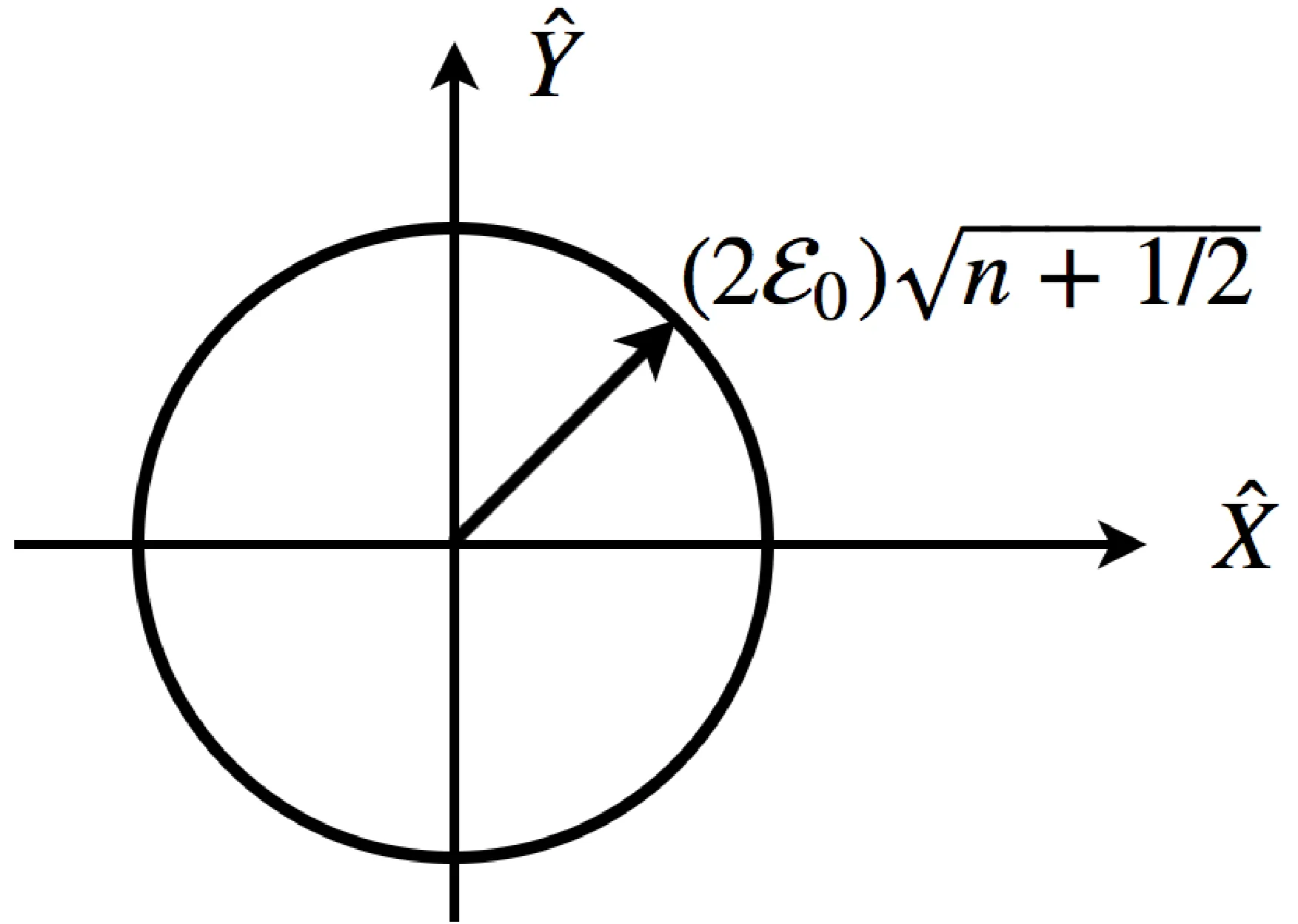
As we have seen, the coherent state is a minimum uncertainty state which have their mean at a particular value of $X$ and $Y$ . This provides a means of plotting states which is called the Husimi-Q function, often shortened to Q function. This is defined for a pure state as

Q (| Ψ ⟩ ⟨ Ψ |, β) = \frac{1}{π} | ⟨ β ∣ Ψ ⟩ |^{2},

where $β$ is a coherent state and the factor of $1 / π$ accounts for the fact that the coherent states are overcomplete. This function is a regular continuous function which is always positive. Integrating over $β$ it gives 1 . Therefore it looks like a probability distribution in classical phase space. In fact this is one of several phase space distributions for quantum oscillators. For a coherent state $α$ the Q function is

\frac{1}{π} | ⟨ α ∣ β ⟩ |^{2} = \frac{1}{π} e^{- | α - β |^{2}} .

2.3.2 Coherent States for Measurement

Classical fields are used in interferometry, for example in a Michelson-Morley interferometer using laser light, which is similar to a coherent state field. Usually, we aim to find the phase difference between two fields in an interferometric setup. The uncertainty of the measurement of the phase angle after the measurement of the quadrature is then of interest, since it limits the interferometer. We can evaluate the uncertainty of the phase of the field as

Δ ϕ = \frac{1 / 2}{| α |} = \frac{1}{2 \sqrt{n}} .

It defines the quantum limit for the measurement of the phase angle of a coherent state. From this value, we can derive an analogous result to the Heisenberg uncertainty relation for the phase and photon number:

Δ n \cdot Δ ϕ = \sqrt{\bar{n}} \cdot \frac{1}{2 \sqrt{\bar{n}}} = \frac{1}{2} .

An important scientific interferometer is the gravitational wave detector LIGO, which enabled the detection of gravitational waves in two MIchelson interferometer.

2.4 Squeezed Light

Heisenberg's uncertainty relation set a limit to the product of the uncertainties of the two quadratures of the field, namely

Δ X \cdot Δ Y \geq \frac{1}{4} in normalized units (2 E_{0} = 1) .

However, in principle nothing prevents the reduction of one quadrature at the expense of the other. Such a light is called quadrature squeezed if

(Δ E (χ))^{2} < \frac{1}{4} .

Consider the squeezed state $| ξ ⟩$ defined by the application of the squeeze operator onto the vacuum,

| ξ ⟩ = \hat{S} (ξ) | 0 ⟩ .

This operator is defined as

\hat{S} (ξ) = \exp (\frac{1}{2} ξ^{*} \cdot {\hat{a}}^{2} - \frac{1}{2} ξ \cdot {({\hat{a}}^{†})}^{2}) with ξ = s e^{i θ},

where $ξ$ is the complex squeeze parameter. The operator $\hat{S} (ξ)$ is unitary, as

{\hat{S}}^{†} (ξ) \hat{S} (ξ) = \hat{S} (ξ) {\hat{S}}^{†} (ξ) = 1 .

The resulting state can be written in the Fock state basis as

| ξ ⟩ = \sqrt{sech (s)} \sum_{n = 0}^{\infty} \frac{\sqrt{(2 n)!}}{n!} {[- \frac{1}{2} e^{i θ} \tanh (s)]}^{n} | 2 n ⟩,

where $sech (s) = 1 / \cosh (s) = 2 / (e^{s} + e^{- s})$ . This state is constructed from even number of photons only. We have as a result

⟨ ξ | \hat{a} | ξ ⟩ = ⟨ ξ | {\hat{a}}^{†} | ξ ⟩ = 0 .

To evaluate $⟨ ξ | {\hat{X}}^{2} | ξ ⟩$ , we will need quantities such as $⟨ ξ | \hat{a} \hat{a} | ξ ⟩$ that will be computed using the following equalities

\begin{aligned} {\hat{S}}^{†} (ξ) \hat{a} \hat{S} (ξ) & = \hat{a} \cosh (s) - {\hat{a}}^{†} e^{i θ} \sinh (s) \\ {\hat{S}}^{†} (ξ) {\hat{a}}^{†} \hat{S} (ξ) & = {\hat{a}}^{†} \cosh (s) - \hat{a} e^{- i θ} \sinh (s) \end{aligned}

by using $e^{- \hat{O}} \hat{a} e^{\hat{O}} = \hat{a} + [\hat{a}, \hat{O}] + \frac{1}{2!} [[\hat{a}, \hat{O}], \hat{O}] + \dots$ . We then find that

\begin{aligned} ⟨ ξ | \hat{a} \hat{a} | ξ ⟩ & = - e^{i θ} \cosh (s) \sinh (s) and ⟨ ξ | {\hat{a}}^{†} {\hat{a}}^{†} | ξ ⟩ = - e^{- i θ} \cosh (s) \sinh (s), \end{aligned}

for $s > 0.$ With this at hand, we find the variance of the quadrature $(Δ \hat{X})^{2}$ as

\begin{aligned} (Δ \hat{X})^{2} & = ⟨ {\hat{X}}^{2} ⟩ - ⟨ \hat{X} ⟩^{2} = \frac{1}{4} (\cosh (2 s) - \cos (θ) \sinh (2 s)), \end{aligned}

and that of the $Y$ quadrature as

(Δ \hat{Y})^{2} = \frac{1}{4} (\cosh (2 s) + \cos (θ) \sinh (2 s)) .

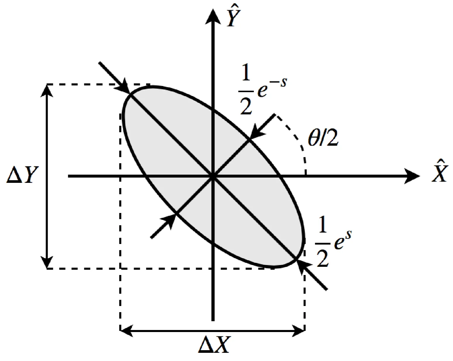
The expectation values and their uncertainties are lying on an ellipse with axes of length $\frac{1}{2} e^{s}$ and $\frac{1}{2} e^{- s}$ inclined at an angle $\frac{θ}{2}$ from the $x$ -axis. Physically, one has squeezed the uncertainty on one quadrature at the expense of the other:

Attachments/QO_Home 1.webp|700

The electric field operator $\hat{E} (χ)$ , that we defined as

\hat{E} (χ) = E_{0} (\hat{a} e^{- i χ} + {\hat{a}}^{†} e^{i χ}) = \hat{X} \cos (χ) + \hat{Y} \sin (χ)

is such that the expectation of the field in the state $| ξ ⟩$ is

⟨ ξ | \hat{E} (χ) | ξ ⟩ = ⟨ ξ | \hat{S} {\hat{S}}^{†} \hat{E} \hat{S} {\hat{S}}^{†} | ξ ⟩ = ⟨ 0 | {\hat{S}}^{†} \hat{E} \hat{S} | 0 ⟩ = 0 .

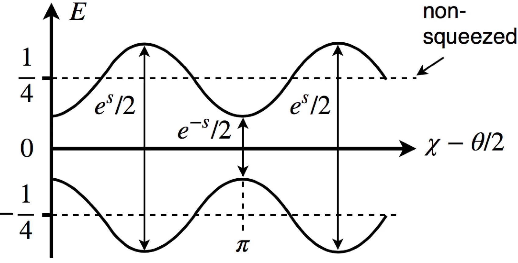
This is not surprising, since it is a squeezed vacuum state. Similarly, the field variance is

(Δ \hat{E} (χ))^{2} = ⟨ (\hat{X} \cos (χ) + \hat{Y} \sin (χ))^{2} ⟩ = \frac{1}{4} (e^{2 s} \sin^{2} (χ - \frac{θ}{2}) + e^{- 2 s} \cos^{2} (χ - \frac{θ}{2})) .

This means that the fluctuations are 'modulated' as a function of the phase angle.

Schematically, it means that the fluctuations are "modulated" as a function of the phase angle. Such squeezed vacuum state can be measured by a homodyne experiment, while the squeezed state can be generated by a non-linear optics process.

Attachments/QO_Home 2.webp|700

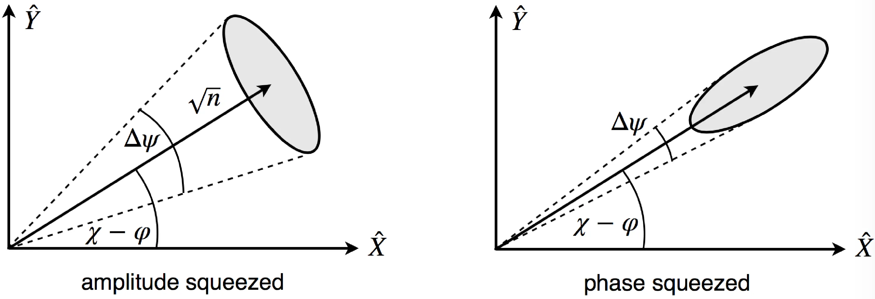
2.4.1 Squeezed Coherent State

Mathematically, a squeezed coherent state can be obtained from a vacuum state by application of a squeeze and displace operator:

| α, ξ ⟩ = \hat{D} (α) \hat{S} (ξ) | 0 ⟩ with \hat{D} (α) = \exp (α {\hat{a}}^{†} - α^{*} \hat{a}) .

Application of this pair of operators lead to the following transformations on the operators $\hat{a}$ and ${\hat{a}}^{†}$

\begin{aligned} {\hat{S}}^{†} {\hat{D}}^{†} \hat{a} \hat{D} \hat{S} & = \hat{a} \cosh (s) - {\hat{a}}^{†} \sinh (s) e^{i θ} + α \\ {\hat{S}}^{†} {\hat{D}}^{†} {\hat{a}}^{†} \hat{D} \hat{S} & = {\hat{a}}^{†} \cosh (s) - \hat{a} \sinh (s) e^{- i θ} + α^{*} . \end{aligned}

We now find that the expectation of the field is non-zero:

\begin{aligned} ⟨ α, ξ | \hat{X} | α, ξ ⟩ & = Re (α) = | α | \cos (φ) and ⟨ α, ξ | \hat{Y} | α, ξ ⟩ = Im (α) = | α | \sin (φ) . \end{aligned}

The uncertainties on $(Δ \hat{X})^{2}$ and $(Δ \hat{Y})^{2}$ are the same as for the vacuum state

(Δ \hat{X})^{2} = \frac{1}{4} (e^{2 s} \sin^{2} (\frac{θ}{2}) + e^{- 2 s} \cos^{2} (\frac{θ}{2})) .

Therefore, the noise measured for a specific phase angle $χ$ is

(Δ \hat{E} (χ))^{2} = \frac{1}{4} (e^{2 s} \sin^{2} (χ - \frac{θ}{2}) + e^{- 2 s} \cos^{2} (χ - \frac{θ}{2})),

while the expectation value is

⟨ α, ξ | \hat{E} | α, ξ ⟩ = | α | \cos (χ - φ) .

The signal over noise is then

SNR = \frac{S^{2}}{N} = \frac{⟨ α, ξ | \hat{E} (χ) | α, ξ ⟩^{2}}{⟨ α, ξ | Δ \hat{E} (χ) | α, ξ ⟩^{2}} = \frac{4 | α |^{2} \cos^{2} (χ - φ)}{e^{2 s} \sin^{2} (χ - \frac{θ}{2}) + e^{- 2 s} \cos^{2} (χ - \frac{θ}{2})} .

The maximum of the SNR is reached for $χ = φ = \frac{θ}{2}$ and yields

{SNR}_{max} = 4 | α |^{2} e^{2 s} .

The average number of photons in that state is

⟨ α, ξ | \hat{n} | α, ξ ⟩ = | α |^{2} + \sinh^{2} (s)

and follows from the additive properties of the displacement and squeeze operator. For states with large relative photon numbers $(| α | ≫ e^{s})$ we have the uncertainty for the photon number $(φ = \frac{θ}{2})$

Δ n = {(\sqrt{⟨ n ⟩} + \frac{1}{4} e^{- s})}^{2} - {(\sqrt{⟨ n ⟩} - \frac{1}{4} e^{- s})}^{2} = \sqrt{⟨ n ⟩} e^{- s},

while the uncertainty on the phase is

Δ ψ = \frac{e^{s}}{2} \frac{1}{| α |} = \frac{e^{s}}{2 \sqrt{⟨ n ⟩}} .

So we have that

Δ n \cdot Δ ψ = \frac{1}{2},

as is expected for minimum uncertainty states. By playing with the value of $s$ , we can enhance or reduce the relative weight of the phase and photon number uncertainty (or by rotating the angle $\frac{θ}{2}$ , of course). This is then called phase-squeezed or amplitude-squeezed, respectively:

Attachments/QO_Home 3.webp|700