Jump back to chapter selection.

Table of Contents

1.1 Maxwell's Equation of Macroscopic Electromagnetism
1.2 Travelling-Wave Solution
1.3 The Dispersion of the Free Electron Gas and Volume Plasmons
1.4 Real Metals and Interband Transitions
1.5 The Energy of the Electromagnetic Field in Metals

1 Electromagnetics of Metals

The interaction of metals with electromagnetic waves can be understood in a classical framework based on Maxwell's equations. This holds true even for metallic nanostructures down to sizes on the order of a few nanometres, without the need to resort to quantum mechanics. This is because the high density of free carriers results in narrow spacings of the electron energy levels compared to the thermal excitation energy $k_{B}T$ at room temperature. This explains why a classical models such as the Drude model or the Maxwell equations are sufficient. It is well known that most metals are highly reflective up to some frequency in the visible range. They are thus traditionally used as cladding layers for constructing waveguides and resonators at microwave and far-infrared frequencies.

In this low-frequency regime, the perfect conductor approximation of infinite or fixed finite conductivity is valid for most purposes since only a negligible fraction of the impinging electromagnetic waves penetrates the metal. However, at higher frequencies approaching the near-IR and visible spectrum, field penetration increases significantly. At UV frequencies, metals acquire a dielectric character and allow the propagation of electromagnetic waves, albeit with varying degrees of attenuation depending on the details of the electronic band structures. Alkali metals, such as sodium, have an almost free-electron-like response and thus exhibit ultraviolet transparency. Noble metals, such as gold and silver, exhibit strong absorption in this regime due to transitions between electronic bands.

1.1 Maxwell's Equation of Macroscopic Electromagnetism

These dispersive properties can be described by a complex dielectric function $\epsilon (\omega )$, which forms the basis of all phenomena discussed.

As a starting point, recall Maxwell's equations of macroscopic electromagnetism:

These equations link the four macroscopic fields:

1. The dielectric displacement $\mathbf{D}$,
2. The electric field $\mathbf{E}$,
3. The magnetic field $\mathbf{H}$,
4. The magnetic induction (or magnetic flux density) $\mathbf{B}$

with the free charge and current densities ${\rho }_{\text{f}}$ and ${\mathbf{J}}_{\text{f}}$. The advantage of this phenomenological approach is that details of the fundamental interactions need not be taken into account since the rapidly varying microscopic fields are averaged over distances much larger than the underlying microstructure.

We distinguish between free (${\rho }_{\text{f}},{\mathbf{J}}_{\text{f}}$) and bound (${\rho }_{\text{b}},{\mathbf{J}}_{\text{b}}$) charge and current densities, so that in total:

and

The four macroscopic fields are further linked via the polarisation $\mathbf{P}$ and magnetisation $\mathbf{M}$:

where ${\epsilon }_0$ and ${\mu }_0$ are the electric permittivity and magnetic permeability of vacuum, respectively. Since we do not treat magnetic media, we will not consider the magnetic response represented by $\mathbf{M}$. Instead, we limit the description to polarisation effects. $\mathbf{P}$ describes the electric dipole moment per unit volume inside the material, caused by the alignment of microscopic dipoles with the electric field. It is related to the bound charge density via:

Charge conservation ($\mathrm{\nabla }\cdot \mathbf{J}=-\frac{\partial \rho }{\partial t}$) further requires that the bound charge and current densities are linked via:

The great advantage of this approach is that the macroscopic electric field includes all polarisation effects: in other words, both the external and induced fields are absorbed into it:

Limiting ourselves to linear, isotropic, and nonmagnetic media, one can define the constitutive relations:

Here, $\epsilon$ is the dielectric constant or relative permittivity, and $\mu =1$ is the relative permeability of the nonmagnetic medium. The linear relationship between $\mathbf{D}$ and $\mathbf{E}$ is often implicitly defined using the dielectric susceptibility $\chi$, which describes the linear relationship between $\mathbf{P}$ and $\mathbf{E}$ via:

The last important constitutive linear relationship to mention is that between the free current density $\mathbf{J}$ and the electric field $\mathbf{E}$, defined via the conductivity $\sigma$ as:

It should be noted that the linear relations for $\mathbf{D}$ and $\mathbf{J}$ are only correct for linear media that do not exhibit spatial dispersion. For media with temporal dispersion, these relations are still linear, however only in frequency-space. The fundamental relation between relative permittivity (from now on called the dielectric function) and conductivity is:

for a given wave vector $k$. From now, we will write $\epsilon ,$ but actually mean the relative permittivity ${\epsilon }_r.$ If the wavelength $\lambda$ is significantly longer than all characteristic dimensions (such as the unit cell size or the mean free path of the electrons), and considering the interaction of light with metals, this equation can be simplified to the limit of a spatially local response, $\epsilon (k=0,\omega )=\epsilon (\omega ).$ In general,

and

are complex-valued functions of angular frequency $\omega$. At optical frequencies, $\epsilon$ can be experimentally determined, for example, via reflectivity studies and the determination of the complex refractive index $\tilde{n}(\omega )=n(\omega )+i\kappa (\omega )$ of the medium, defined as:

Explicitly, this leads to the components of the dielectric function:

Here, $\kappa$ is called the extinction coefficient and determines the optical absorption of electromagnetic waves propagating through the medium. It is linked to the absorption coefficient $\alpha$ of Beer’s law (describing the exponential attenuation of the intensity of a beam propagating through the medium via $I(x)=I_0{e}^{-\alpha x}$) by the relation:

Therefore, the imaginary part ${\epsilon }_2$ of the dielectric function determines the amount of absorption inside the medium. For $|{\epsilon }_1|\gg |{\epsilon }_2|$, the real part $n$ of the refractive index, which quantifies the lowering of the phase velocity of the propagating waves due to the polarisation of the material, is mainly determined by ${\epsilon }_1$. The real part of $\sigma$ determines the amount of absorption, while the imaginary part contributes to ${\epsilon }_1$ and therefore to the amount of polarisation.

1.2 Travelling-Wave Solution

When studying the propagation of wave in vacuum, the focus is always on transverse waves, as longitudinal solutions do not exist . This is no longer the case in a medium. Plasmons are longitudinal solutions of the Maxwell equations. By considering the propagation of coupled mechanical and electromagnetic waves, the electromagnetic solution has an electric parallel to the wavevector. More generally, this solution is a longitudinal solution with

Therefore, such an equation is fully described by

Let us examine the existence of a longitudinal solution of Maxwells equation without invoking a specific model of the medium. We will only assume, as always, a linear, homogeneous and isotropic medium, such that we can use the dielectric function:

Note that the frequency dependence of the dielectric function is called dispersion, while its dependence on the wavevector is called spatial dispersion. By considering the relation in real space, and invoking the zero divergence of the displacement field, we find that we can differentiate two cases:

• Longitudinal waves: Seeking a non-zero longitudinal electric field, we impose $\mathbf{K}\cdot \mathbf{E}(\mathbf{K},\omega )\ne 0.$ This then leads to

  $$\epsilon (\mathbf{K},\omega )=0,$$

  which can be further simplified to $\epsilon (\omega )=0$ for a local medium. This signifies that longitudinal collective oscillations can only occur at frequencies corresponding to zeros of $\epsilon (\omega )$. Indeed, one such solution is $\omega ={\omega }_p$ in the case of a non-lossy Drude model. Keep in mind, neglecting the $\mathbf{K}$-dependence typically holds well for $K\ll {\omega }_p/k_F.$ The Drude model is inherently a local model, that makes this assumption.

• Transverse waves, $\mathbf{K}\cdot \mathbf{E}=0$, resulting in the generic dispersion relation:

  $$K^2=\epsilon (\mathbf{K},\omega )\frac{{\omega }^2}{c^2}.$$

1.3 The Dispersion of the Free Electron Gas and Volume Plasmons

Let us discuss the transparency regime $\omega >{\omega }_p$ of the free electron gas model. For that, consider the Lorentz-Drude model. The dispersion of the travelling waves is:

This relation is plotted here:

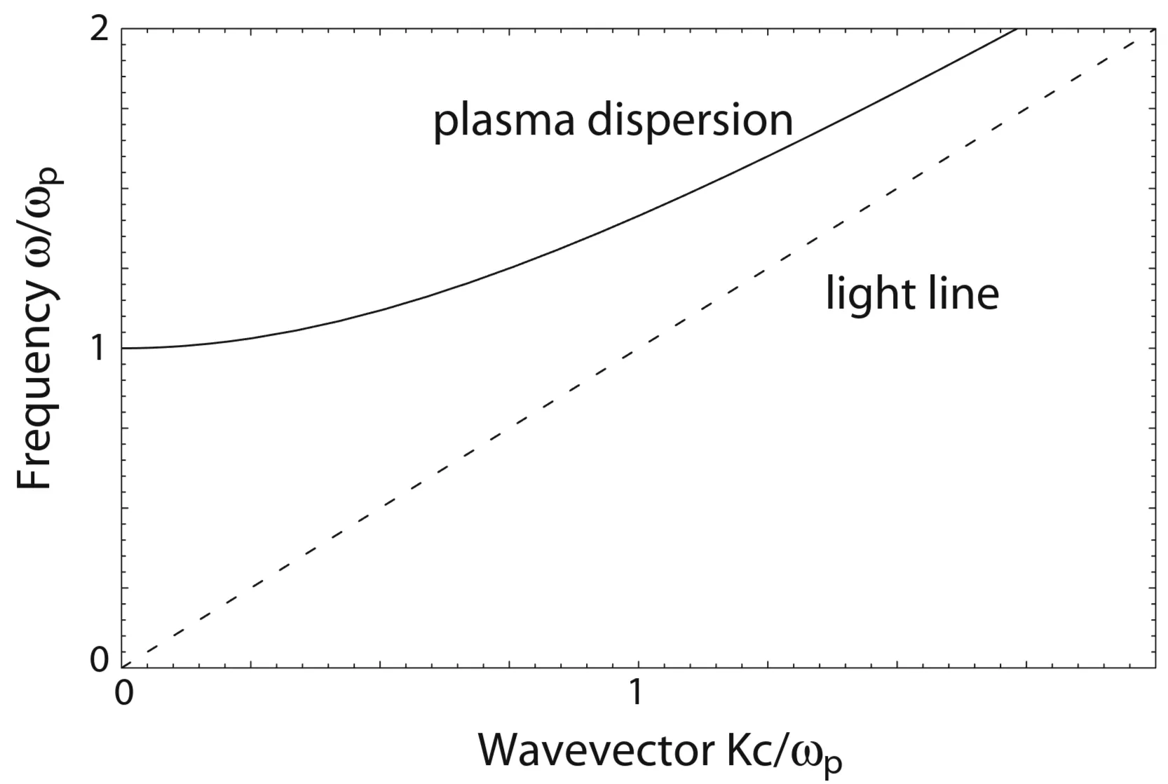
For frequencies below the plasma frequency, the propagation of transverse electromagnetic waves is forbidden inside the metal plasma. For larger frequencies, however, the plasma supports transverse waves propagating with a group velocity $v_g=d\omega /dK<c$. Noting that $\epsilon (K=0,{\omega }_p)=0$, the excitation must correspond to a collective longitudinal mode. At the plasma frequency, the electric field is a pure depolarisation field.

The physical significance of this excitation at the plasma frequency can be understood by considering the collective longitudinal oscillation of the conduction electron gas against the fixed positive background of the ion core in a plasma slab:

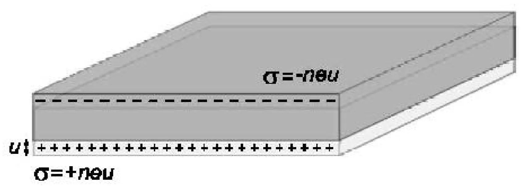
A collective displacement of the electron cloud leads to a surface charge density at the slab boundaries. This establishes a homogeneous electric field inside the slab. Therefore, the displaced electrons experience a restoring force, and the plasma frequency is the natural frequency of a free oscillation of the electron sea. This assumes all electrons move in phase, meaning the plasma frequency corresponds to the oscillation frequency in the long-wavelength limit where $K=0$.

The quanta of these charge oscillations are called volume plasmons, to distinguish them from surface and localised plasmons. Due to the longitudinal nature of the excitation, volume plasmons do not couple to transverse electromagnetic waves and can only be excited by particle impact. Another consequence of this is that their decay occurs mainly via energy transfer to single electrons in collisionless plasmas, a process known as Landau damping.

In addition to the in-phase oscillation at ${\omega }_p$, there exists a whole class of longitudinal oscillations at higher frequencies with finite wave vectors, for which $\epsilon (K,\omega )=0$ is fulfilled:

1.4 Real Metals and Interband Transitions

As already mentioned, the dielectric function of the Drude model adequately describes the optical response of metals only for photons below the transition energy between electronic bands. For some noble metals, interband effects already occur around $1$ eV ($\lambda \approx 1\mu \mathrm{m}$). In silver for example, the interband absorption edge is around $3.8$ eV:

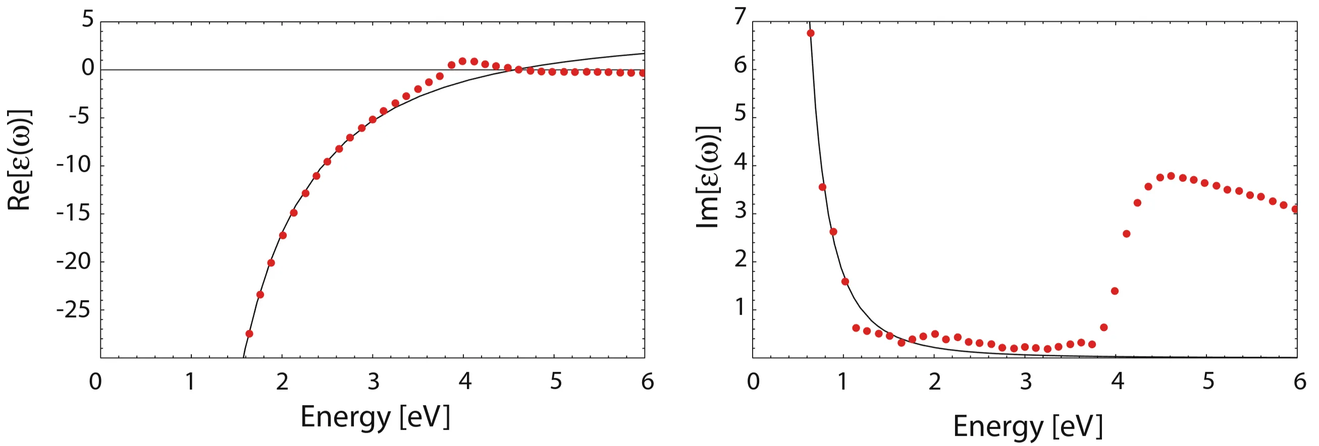
The red dots are experimentally obtained results, while the line is a fit of the Drude model. Clearly, the model is not adequate to describe either the real or imaginary part of the dielectric function at high frequencies, and in the case of gold, its validity already breaks down close to the visible range.

1.5 The Energy of the Electromagnetic Field in Metals

For a linear medium with no dispersion or losses, the total energy density of the electromagnetic field can be written as:

This expression, together with the Poynting vector of energy flow $\mathbf{S}=\mathbf{E}\times \mathbf{H}$, enters into the conservation law (Poynting's theorem):

relating changes in electromagnetic energy density to energy flow and Ohmic losses (work done by the field on free charges) inside the material.

However, in metals, the dielectric function ${\epsilon }_r(\omega )$ is complex and strongly frequency-dependent due to dispersion and absorption. Consequently, the simple expression for the total energy density $u$ in the form above does not directly apply. For dispersive media, the energy stored in the electric field is not solely determined by the instantaneous field strength but also depends on the history of the field, or equivalently, on the frequency response of the material.

A more general expression for the time-averaged electric energy density in a dispersive, low-loss medium, when the electric field $\mathbf{E}(\mathbf{r},t)$ is appreciable only in a narrow frequency range around a central frequency ${\omega }_0$ and varies slowly compared to a timescale $1/{\omega }_0$, is given by:

where ${\epsilon }_1(\omega )=\mathfrak{Re}[{\epsilon }_r(\omega )]$, and $|\mathbf{E}(\mathbf{r}){|}^2$ represents the square of the peak amplitude of the time-harmonic electric field (so if $\mathbf{E}(\mathbf{r},t)=\mathfrak{Re}[\mathbf{E}(\mathbf{r})e^{i{\omega }_{0}t}]$, then $|\mathbf{E}(\mathbf{r}){|}^2$ is the peak amplitude squared). The requirement of low absorption (so $|{\epsilon }_2|\ll |{\epsilon }_1|$, where ${\epsilon }_2=\mathfrak{Im}[{\epsilon }_r(\omega )]$) limits the applicability of this specific form, for example, to visible and near-infrared frequencies for some metals, but not necessarily to lower frequencies or within regions of strong interband absorption where $|{\epsilon }_2|$ can be comparable to or greater than $|{\epsilon }_1|$.

However, the electric field energy can also be determined by explicitly considering the electric polarisation. For a material described by a free-electron-type (Drude model) dielectric function ${\epsilon }_r(\omega )={\epsilon }_1(\omega )+i{\epsilon }_2(\omega ),$ the time-averaged effective electric energy density is given by:

where $\gamma$ is the damping rate from the Drude model. The factor of $1/4$ (rather than $1/2$) arises from time-averaging a harmonically oscillating field and using the peak amplitude squared $|\mathbf{E}(\mathbf{r}){|}^2$. It can be shown that for negligible losses (so small ${\epsilon }_2$ or $\gamma \to 0$), this expression reduces, as expected, to the previous general form for low-loss dispersive media for time-harmonic fields.