Jump back to chapter selection.
Table of Contents
5.1 Proof of Schottky's Theorem for Shot Noise
5.2 Modulation Instabilities
5.3 Autocorrelator
5.4 Diagnostics Measurements
5.5 Welch's Method to Obtain Power Spectral Density Estimates
5 Appendix
The purpose of this appendix is to offer additional context on certain topics that were considered too extensive to include in the main body of this thesis. Given that the primary focus of this thesis is experimental, theoretical aspects, including derivations and proofs, are provided here for completeness.
5.1 Proof of Schottky's Theorem for Shot Noise
Schottky's theorem is a fundamental result in electronics, stating that the shot noise power spectral density (PSD) is proportional to the average current.
Proof
While current flow appears continuous, the discrete nature of charge carriers (such as electrons) leads to random arrival times at the detector, which can be modelled as a Poisson process. The current arriving at the detector at any given time can be expressed as
where
where the autocorrelation function is defined as
Applying this to the problem, with
Evaluating the integral:
This leads to
Care must be taken when evaluating this expression. For
Thus, we are left with
where
This concludes the proof.
It is worth noting that this result holds even if the current pulses are not modelled as delta functions but as square pulses. If the pulses have a duration
While this expression differs from the earlier result, it is important to consider that
5.2 Modulation Instabilities
To begin the discussion, it is essential to recognise that the nonlinear coefficient,
where
Consider a continuous wave (CW) centred around
where the field normalisation ensures that the absolute square of the amplitude represents the power in the fibre. This leads to a nonlinear phase shift:
Next, we express the electric field as a perturbation:
where the perturbation
Thus, the NLSE for the perturbation
where the dispersion term is defined as:
If
The eigenvalues of the resulting coupling matrix indicate the gain for spectral sidebands at frequency shifts of
which reduces to:
in the standard case where only second-order dispersion is considered,
By defining
The parameter
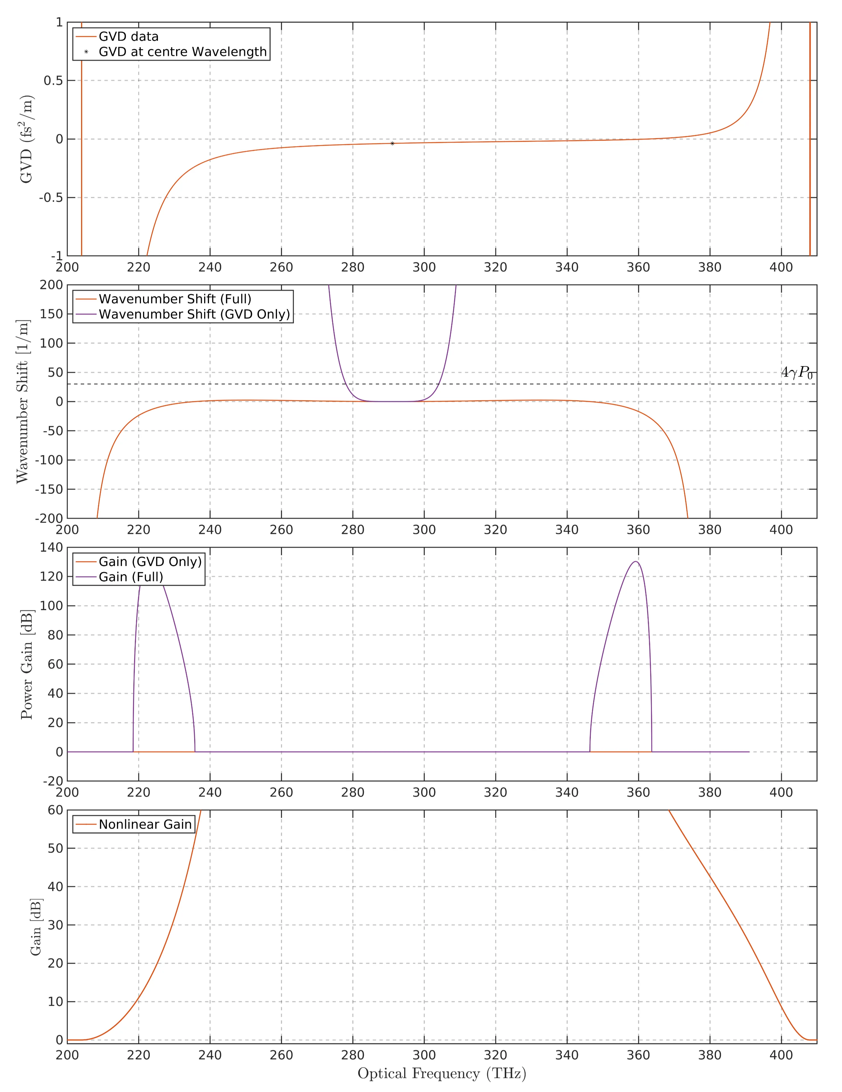
Overview of modulation instabilities in the fibre. (a) The group velocity dispersion (GVD) data shows the raw GVD values across different optical frequencies, with a marker at the centre wavelength highlighting the GVD used in calculations. (b) Wavenumber shift as a function of optical frequency, comparing the full model and the model considering only the GVD contribution. The horizontal dashed line represents the constant term
5.3 Autocorrelator
As pulse durations become shorter than
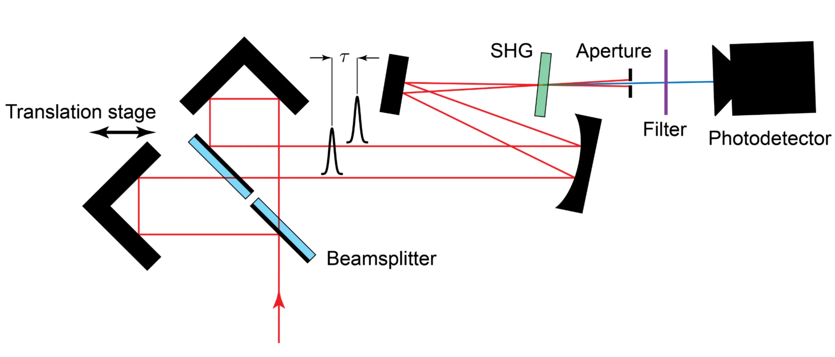
In this method, a beamsplitter divides the incident laser beam into two beams of identical intensity. One of the beam paths is delayed relative to the other by a time
It can be shown that the SHG signal is minimal when the pulses do not overlap temporally and reaches a maximum when they are perfectly overlapped in time. Due to momentum conservation and the non-collinear configuration of the incident beams, the frequency-doubled signal appears spatially between the two original beams. An aperture can be used to isolate and measure only the SHG signal's intensity:
Since this intensity is symmetric with respect to the delay, that is,
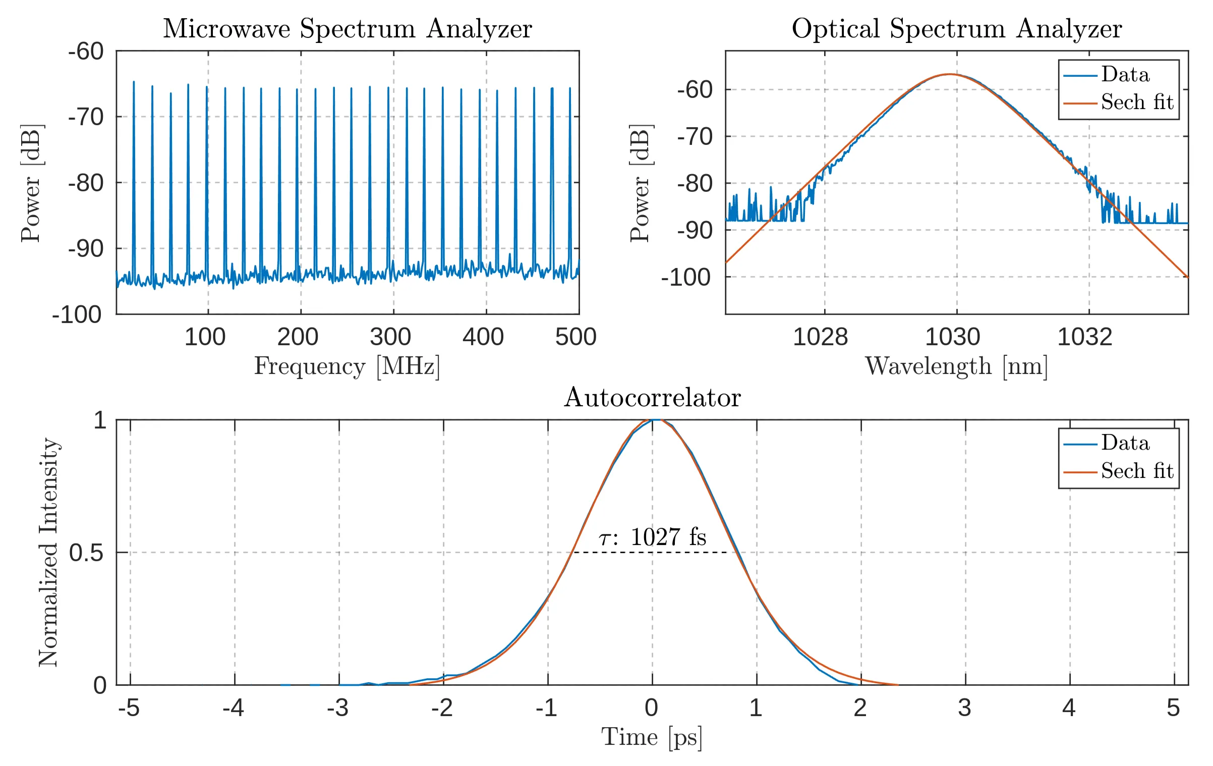
5.4 Diagnostics Measurements
This section presents various measurements from the optical spectrum analyser (OSA), microwave spectrum analyser (MSA), and autocorrelator for completeness. The results are shown in Figures 4.3 to 4.5.
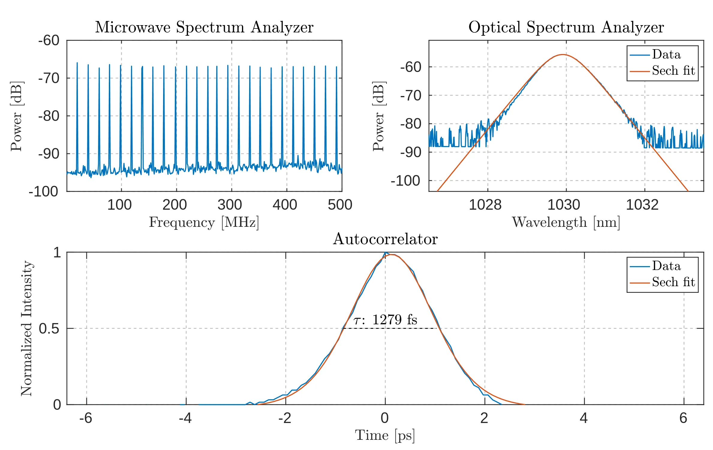
Combined diagnostic results from the microwave spectrum analyser (MSA) with a resolution bandwidth of
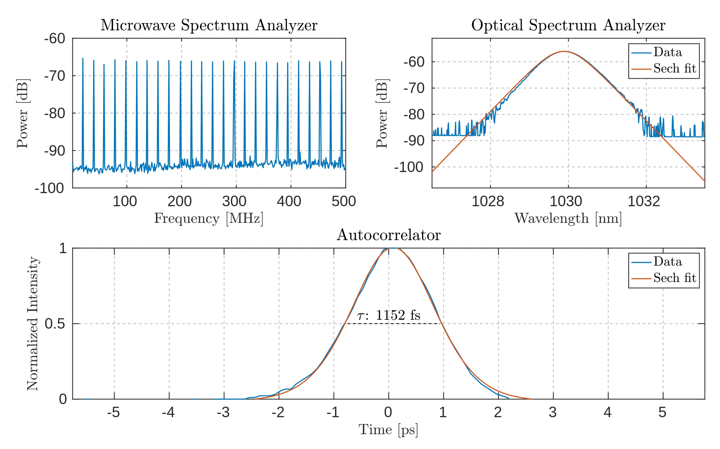
Combined diagnostic results from the microwave spectrum analyser (MSA) with a resolution bandwidth of
Combined diagnostic results from the microwave spectrum analyser (MSA) with a resolution bandwidth of
5.5 Welch's Method to Obtain Power Spectral Density Estimates
As described in Section 3.5.3, Welch's method was employed to smooth the noise PSD data and provide visual clarity. Welch's method is a widely-used approach for estimating the power spectral density of a signal. Unlike a basic periodogram, which can be noisy and less reliable due to its high variance, Welch's method provides a smoother and more reliable estimate by averaging multiple periodograms of overlapping data segments. The initial noise in the data results from the fact that the experiment was conducted with a finite sampling rate and over a finite measurement time. If both the sampling rate and time were infinite, the resulting curve would appear smooth, as the non-stationary signal components would diminish. The process of Welch's method can be broken down into the following steps:
- The signal is divided into 100 overlapping segments, with an
overlap used between successive segments. Overlapping reduces information loss at the segment boundaries and provides more samples for averaging. - A window function, in this case a Hann window, is applied to each segment to minimise spectral leakage. This reduces spectral leakage by avoiding sharp discontinuities at the segment boundaries.
- For each windowed segment, the Fast Fourier Transform (FFT) is used to compute the periodogram, which provides the PSD estimate for that segment.
- Finally, the periodograms of all segments are averaged to produce the overall PSD estimate, reducing variance and creating a smoother representation of the spectral density.
The main strength of Welch's method lies in its ability to reduce the variance of PSD estimates. Compared to a single periodogram, Welch's method is much less sensitive to fluctuations in the data, offering a more stable and reliable representation of the signal's frequency content. In this thesis, it was employed to reveal the shot-noise limit and distinguish the signal from noise in the high-power laser system. However, the primary trade-off is a reduction in frequency resolution. Additionally, Welch's method increases the computational load, as the FFT must be applied multiple times across the overlapping segments.