Jump back to chapter selection.
Table of Contents
3.1 Oscillator
3.2 Beam Diagnostics
3.3 Fibre Coupling
3.4 Grating Spectrometer
3.5 Characterisation
3.6 Technical Considerations
3.7 Full Setup
3 Setup, Characterisation and Results
This chapter discusses the thesis's experimental setup, including the design of the oscillator, fibre coupling, grating spectrometer, and noise measurement techniques. The steps are discussed in the order of the beam path, starting from the laser cavity and ending in the detection setup.
3.1 Oscillator
The cavity design employs a two-pass geometry to achieve a repetition frequency of
The choice of repetition rate is crucial and not arbitrary. A higher repetition rate allows for noise measurements to extend to higher frequencies but also results in lower pulse energies and peak powers, which is not ideal for achieving significant spectral broadening. Conversely, a lower repetition rate enhances spectral broadening due to the increased pulse energies and peak powers; however, it limits noise measurements by restricting the maximum frequency components that can be effectively measured. Thus, a repetition rate of about
The repetition frequency is determined by the distance from the output coupler to the end mirror,
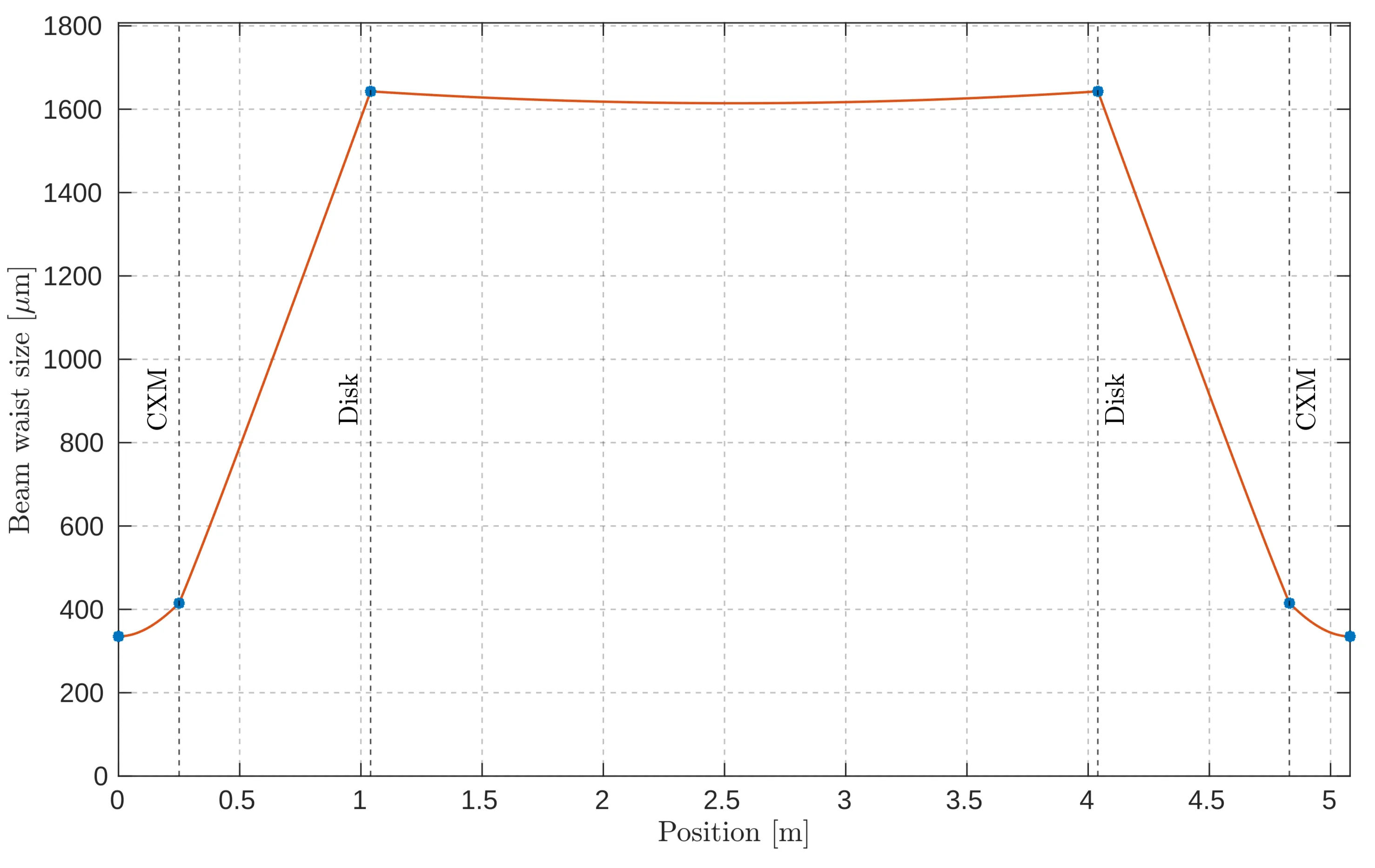
Evolution of the beam waist size (orange) within the simplest two-pass cavity in a symmetric configuration. The black dashed vertical lines and blue dots denote curved mirrors or the disk, with a nominal radius of curvature of
From this starting point, parameters such as distances between mirrors are adjusted, and additional mirrors are added to fit our needs. For stability, the beam must always focus at the ends of the cavity to maintain the periodicity of the beam waist.
To achieve soliton mode-locking, sufficient self-phase modulation is needed to counteract the group delay dispersion. The B-integral quantifies the SPM:
There is no additional SPM medium in the cavity, which is unique compared to most low-power, non-thin-disk lasers that achieve significant self-phase modulation (SPM) within the gain medium, as SPM through air propagation is negligible. In contrast, high-power TDLs usually require a vacuum to reduce undesirable SPM effects. For stable mode-locking, a B-integral around
The next figure shows the final configuration of the TDL cavity, featuring a telescope to control the beam size on the SESAM and, consequently, the fluence on the SESAM. Group Delay Dispersion is introduced using Gires-Tournois interferometer style (GTI) mirrors. These mirrors, while often named after the classical GTI with an air gap, are chirped mirrors. They achieve the desired wavelength-dependent phase shift through a carefully designed, wavelength-dependent optical path difference.
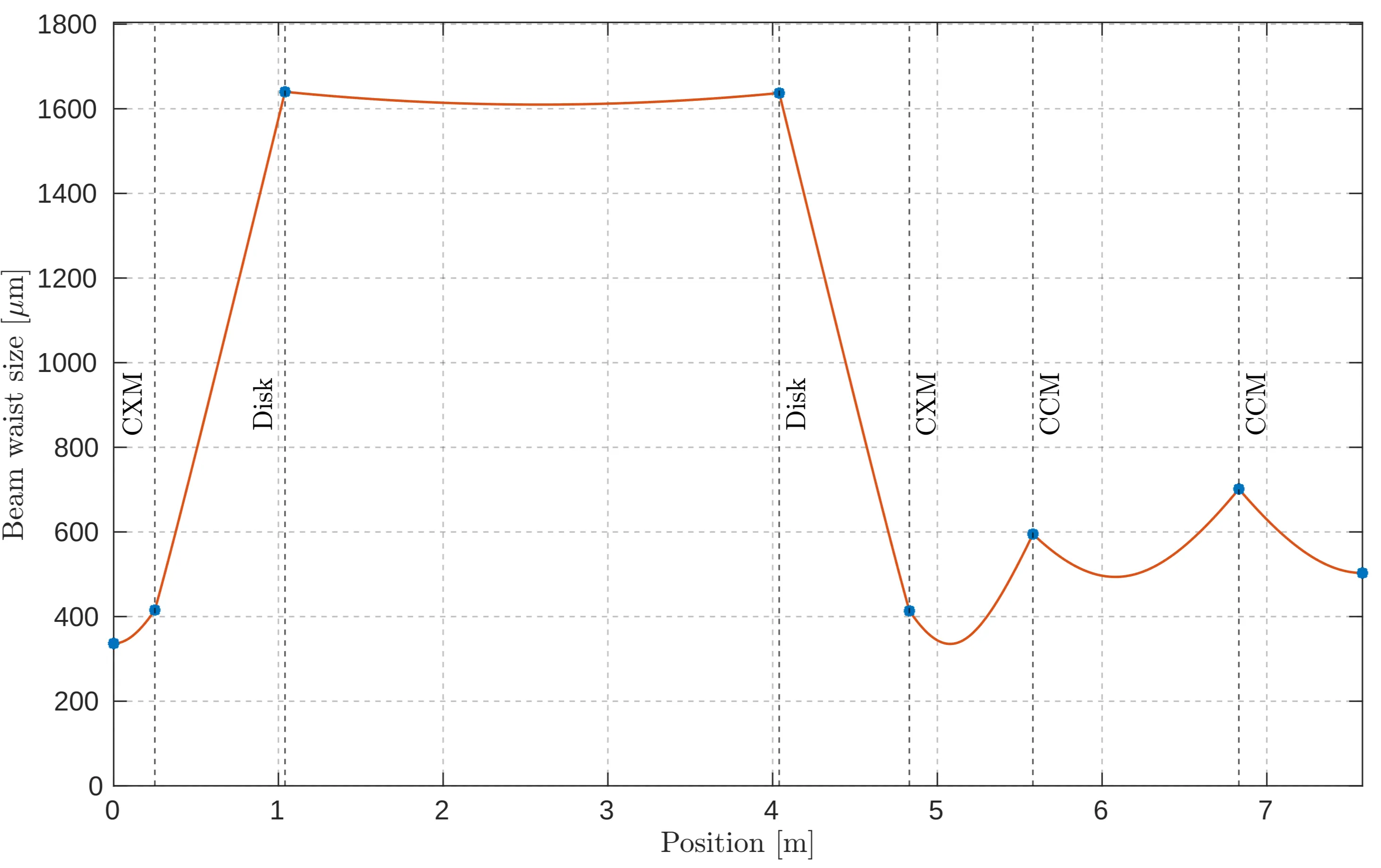
Beam waist evolution in the final cavity configuration, illustrating the change in beam waist size as the light travels through the cavity, starting from the output coupler and ending at the SESAM. Curved mirrors, the TDL disk, SESAM and OC are depicted with blue dots. Plane mirrors and plane GTIs are not shown.
Long-term stability in high-power oscillators also necessitates careful management of thermal effects, as increased power enhances both thermal lensing and disk bending. These effects result in a temperature-dependent radius of curvature, influenced by heating and gas convection in front of the disk. Thermal lensing and gas convection effects are equally significant in an air-filled cavity. The cavity must operate in a regime where small variations in the disk's curvature do not lead to destabilisation. As shown in the next figure, no nearby singularities indicate a stable configuration:
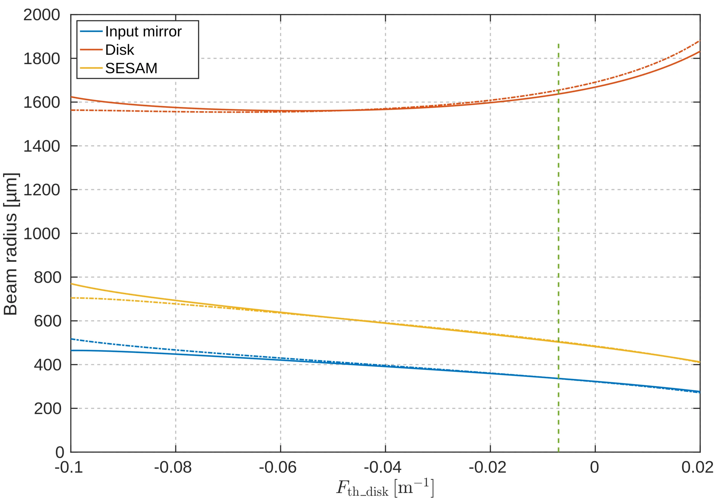
Beam radius on the SESAM as a function of its thermal lensing. The horizontal axis covers a very broad range, fully encompassing the laser's operating range. The absence of singularities or rapid changes suggests a stable configuration with respect to thermal lensing. The operation point of the cavity is depicted as a dashed line.
The following schematically depicts the final cavity configuration. To control the polarisation of the laser output, a thin-film polariser is introduced into the cavity. This ensures that only light with a well-defined polarisation can oscillate, improving the overall beam quality and stability of the cavity.
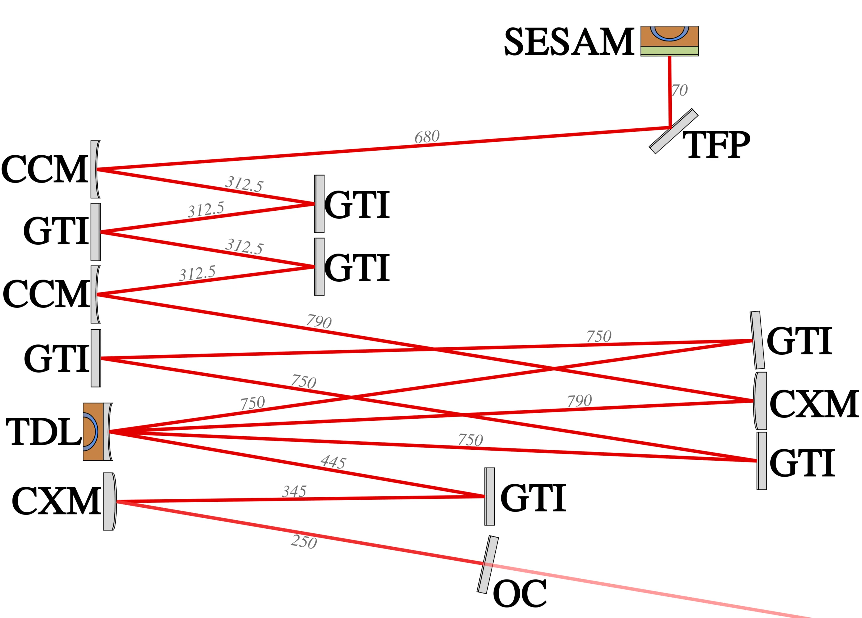
Schematic of the laser cavity and its components. GTI denotes the Gires-Tournois interferometer, TFP represents the thin-film polariser, OC is the output coupler, CCM is the concave mirror, CXM is the convex mirror, and TDL stands for the thin-disk laser. The blue elements behind the SESAM and TDL indicate active water cooling. The path of the oscillating light is shown schematically, with distances in millimetres marked in grey.
The efficiency of the laser system is crucial for evaluating its performance. The output power
where
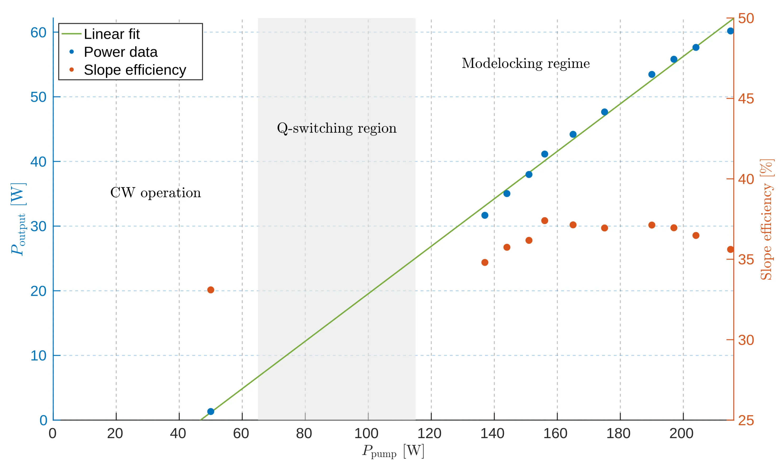
Output power (left) and slope efficiency (right) of the thin-disk laser as a function of pump power. The first data point is before mode-locking has been achieved, while the grey-shaded area is the Q-switching regime (
The next table shows the parameters of this laser cavity.
| Parameter | Value |
|---|---|
| Average output power (no CW breakthrough) | |
| Pulse duration | |
| Repetition rate | |
| Required GDD to counteract SPM | |
| Central wavelength |
3.2 Beam Diagnostics
3.2.1
After the laser light exits the cavity, it is crucial to characterise the output beam quality. A small fraction of the laser power is extracted and directed towards the diagnostics setup. The key metric for beam quality is the
The next figure presents the results of the
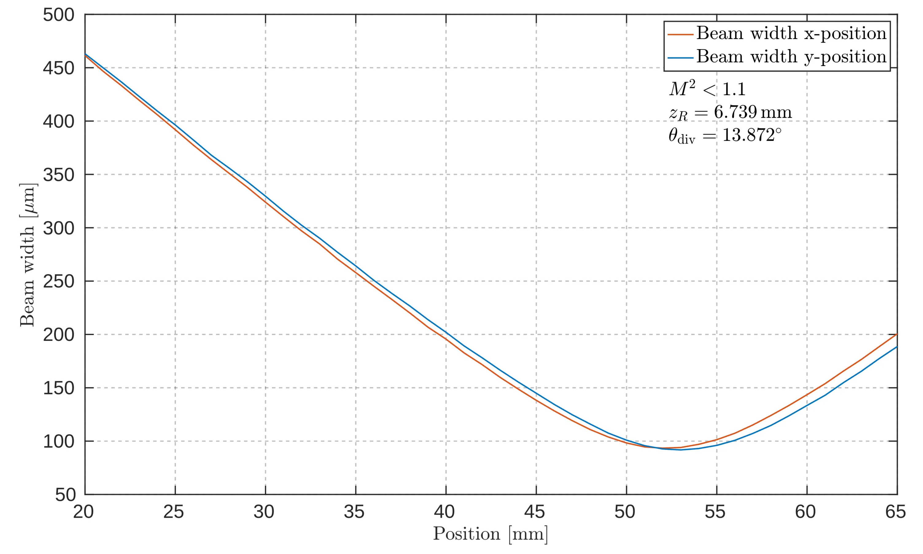
Results of the
3.2.2 Spectrum Analyser
A small portion of the output power, approximately
Another small fraction of the laser power is directed to a microwave spectrum analyser (MSA) to obtain the frequency spectrum, which includes multiple harmonics of the mode-locked signal. A photodiode converts the optical signal into an electrical one for analysis by the MSA. s expected, as shown in the next-next figure, multiple peaks corresponding to harmonics of the repetition rate,
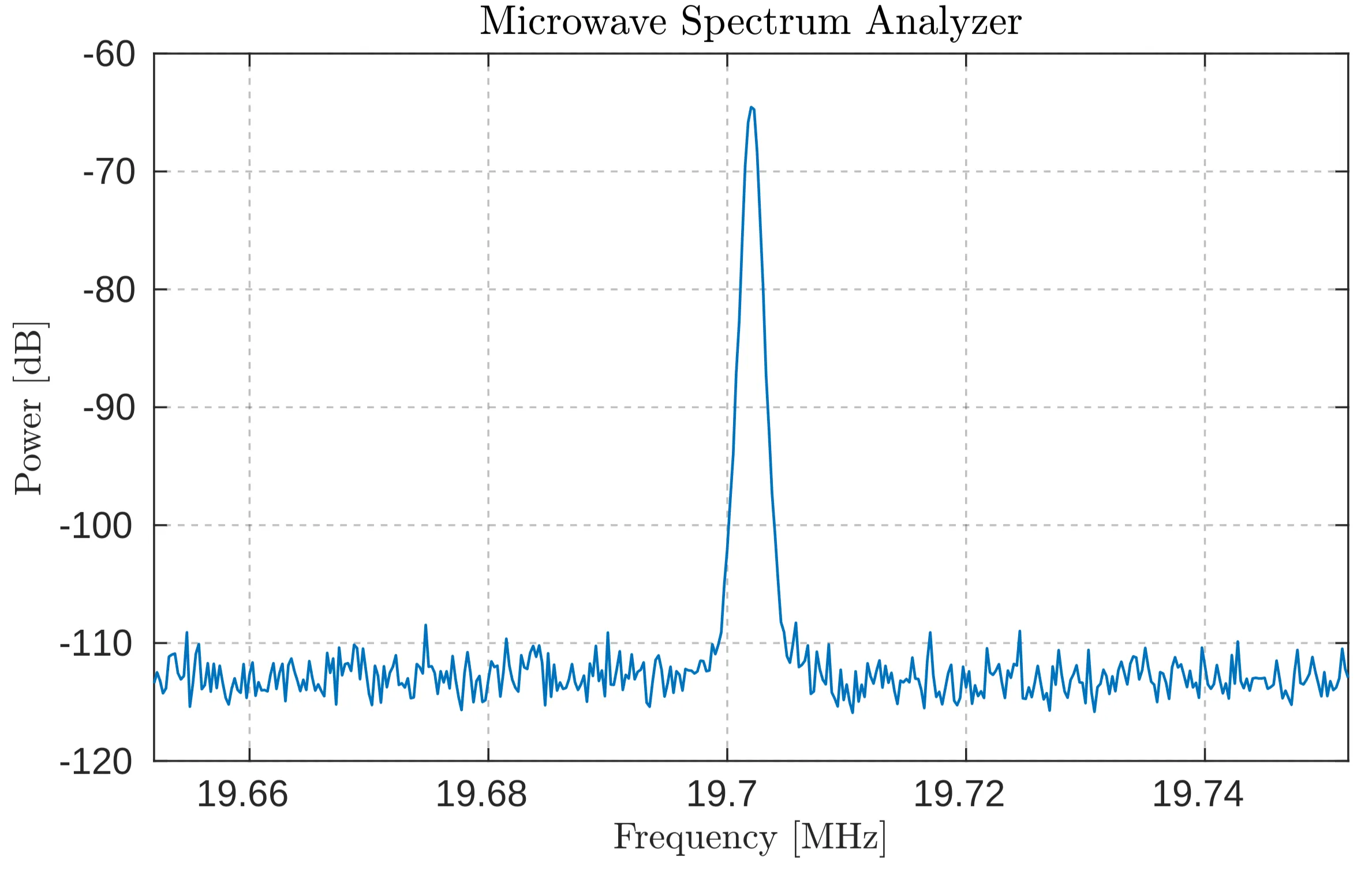
Further diagnostic measurements at different pump powers are detailed in the appendix.
3.2.3 Autocorrelation
We use an intensity autocorrelator to determine the pulse width and the temporal structure of the laser output. The methodology and principles behind this technique are discussed in detail in the appendix. The measured pulse width is approximately
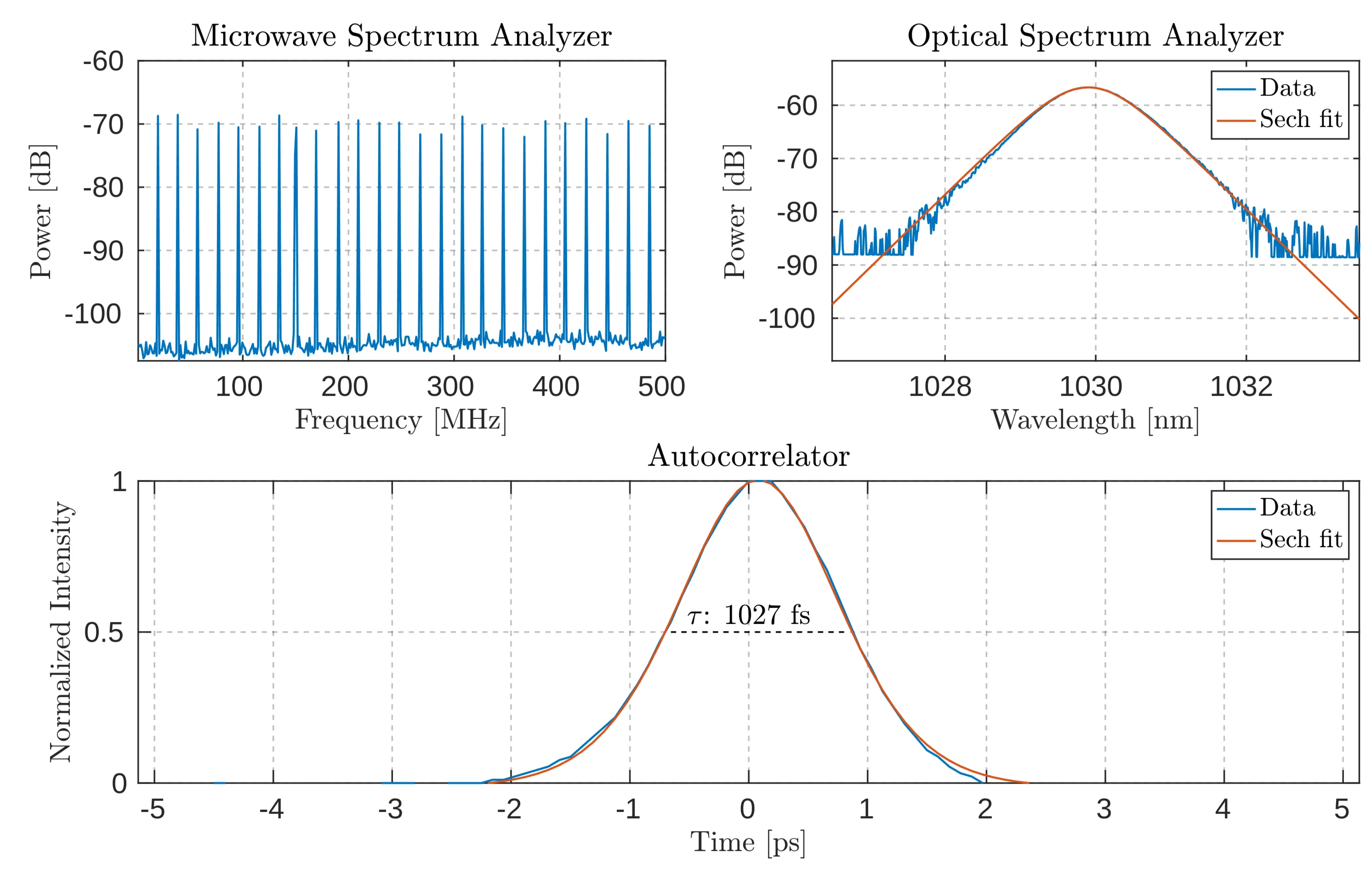
Combined diagnostic results from the microwave spectrum analyser (MSA) measured with
3.3 Fibre Coupling
In this section, the path from the laser cavity to the hollow-core fibre is traced and explained in detail.
3.3.1 Mode-Field Diameter
The specified mode-field diameter (MFD) of the fibre is
Two lenses should have focal lengths with an absolute ratio of 4:3. However, to avoid creating a focus between these two lenses (which could introduce additional artefacts due to high intensity), a combination of convex and concave lenses is used. This is realised using
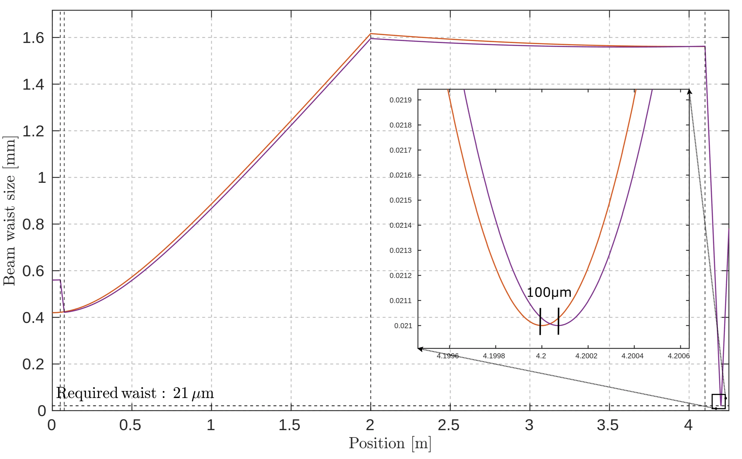
Beam waist evolution as the laser passes from the output coupler of the cavity through the telescope, which optimises the beam for fibre coupling. The orange and violet curves represent the beam waist sizes in the horizontal and vertical axes, respectively. The zoomed-in section highlights slight astigmatism between the horizontal and vertical foci at the fibre's focal point.
The simulation suggests that this setup introduces slight astigmatism, with a spacing of roughly
3.3.2 Power Tuning
Another important consideration is power tuning. Even if everything works as expected, it is dangerous to immediately send full power into the fibre, especially if beam stabilisation has not yet been achieved. A common issue with SESAMs is Q-switching: initially, the output power can be finely tuned from
3.3.3 Polarisation
While the fibre has no defined birefringence, induced birefringence effects along preferential polarisation angles might occur due to the non-radially symmetric structure of the photonic crystal in the fibre and fibre bending. Indeed, the input polarisation can change the beam shape and far-field profile. Incorrect polarisation also dramatically increases the fibre's sensitivity to touch. Therefore, a half-wave plate is placed before the fibre to control the input polarisation.
3.3.4 Fibre Coupling
As mentioned earlier, the specified MFD of the fibre is
3.3.5 Pressure and Gas System
The simulations assume a pressure of
3.4 Grating Spectrometer
As discussed in Section 2.6, applying high pressure to a gas with a high nonlinear refractive index and allowing the pulse to propagate will generally lead to significant spectral broadening. For example, a pulse that initially had a full-width at half-maximum (FWHM) of
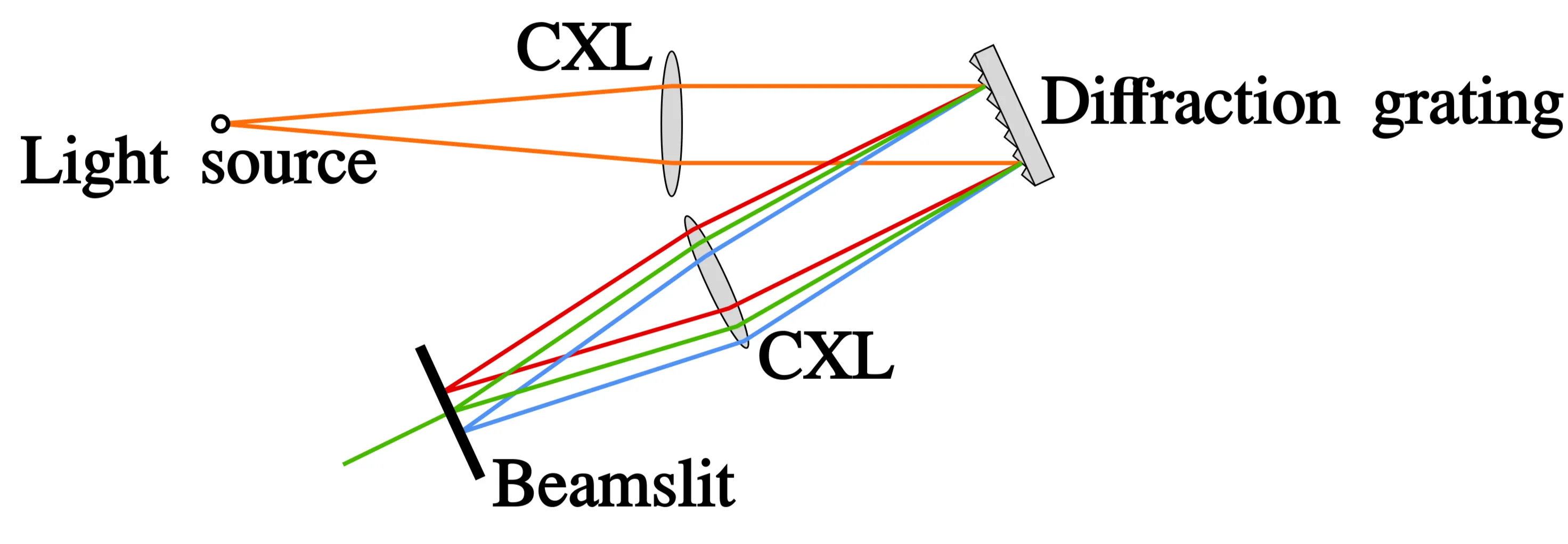
Schematic diagram of a grating spectrometer. The convex lens (CXL) focuses the incoming light and resolves the spectral overlap, allowing each wavelength to be detected at distinct positions on the detector.
A grating functions by altering the incident phase and amplitude of incoming light to separate different wavelengths. The interference pattern created depends on the grating's geometry. In this thesis, a blazed grating is used, characterised by its blaze wavelength, groove spacing
The grating equation relates the angle of incidence
No diffraction pattern is observed in the zeroth order mode (
At twice the blaze angle, we find:
A special case is the so-called Littrow configuration, where the grating efficiency is maximised. This occurs when
where
The angular dispersion
Next, we analyse the free spectral range. Reflected light of different orders may overlap, but this can be avoided for the wavelength range
holds for
Another crucial factor is the spectral resolution, which limits the minimum wavelength differences that can be resolved by using a diffraction grating. There are two approaches to determine whether two wavelengths can be resolved:
-
Resolving Power: The resolving power is defined as
, where is the smallest resolvable difference from , and is the number of illuminated grooves. This allows us to estimate: where
is the beam waist on the grating, is the angle of incidence, and the factor of 2 accounts for the beam waist being a radius. With the beam size of this TDL, this results in a spectral resolution below for a grating with and a Littrow angle of . The next figure shows the beam waist after the fibre, demonstrating that the chosen setup with lenses results in a collimated beam on the grating, justifying the approximation of ignoring the Gaussian nature of the beam.
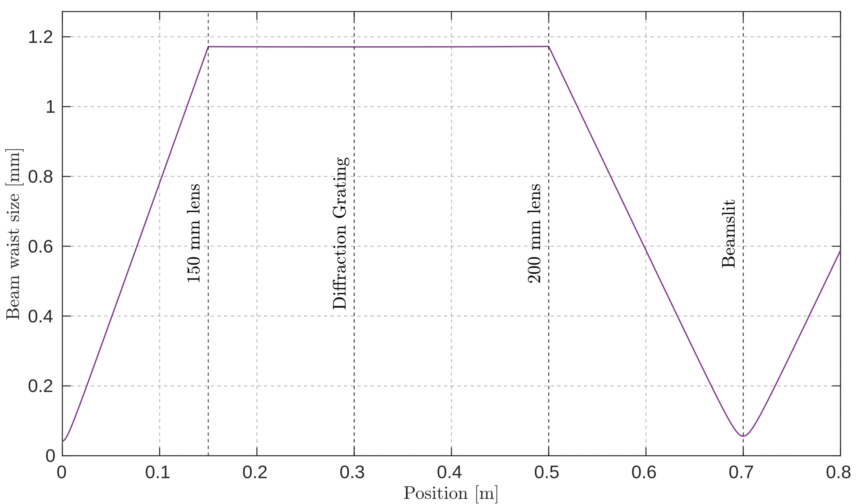
Evolution of the beam waist after exiting the fibre and passing through afocusing lens, which collimates the beam to a large radius at the grating. The beam slit is positioned at the focal point after reflection from the grating to select a specific wavelength range. -
Gaussian Optics: First, assume the grating behaves like an ordinary mirror, not affecting the beam waist. Then, ray transfer matrix analysis simulation shows that the focus behind the second lens will have a waist
. Now, consider the problem: If this behaviour holds for every spectral component, what must be the wavelength difference for their positions in the focus after the lens to differ by ? The spectrum will not be smeared if their separation is larger than their individual waist sizes. This problem simplifies near the Littrow configuration, as the projection of two spots from two spectral components onto a common surface is equal, even for different spectral components. The spatial distance between two wavelengths is: where
is the diffraction angle for a given wavelength and incident angle , and is the focal length of the lens after the grating. Setting , we obtain: which is approximately
. Since this value is lower than the resolution obtained using the resolving power, smearing due to the Gaussian nature of the beam is unlikely to be problematic, as the resolving power would not have permitted higher resolution in the first place.
In summary, this setup allows resolving spectral features as small as
3.5 Characterisation
To fully characterise the laser noise, several key factors must be considered. Firstly, the photodiode (PD) must operate within its linear range, where its voltage response remains proportional to the incident power and does not become saturated. A low-pass filter might be necessary to suppress peaks at the repetition frequency, preventing potential damage to the oscilloscope or signal spectrum analyser.
Suppose amplifiers are employed to enhance the signal. In that case, verifying that they provide consistent gain across the relevant frequency range is essential, meaning they should have a flat frequency response. Additionally, the repetition rate must not exceed the amplifiers' saturation limits. Since consistent gain is typically achievable only within specific frequency bands, multiple amplifiers might be required for different measurements, and their results may need to be combined at a common reference point.
3.5.1 Photodiode Characterisation
Two photodiodes were evaluated for measuring the laser noise: Thorlabs' large-area (
To assess the performance of the photodiodes, the average generated voltage response was measured against the incident power. The generated voltage was
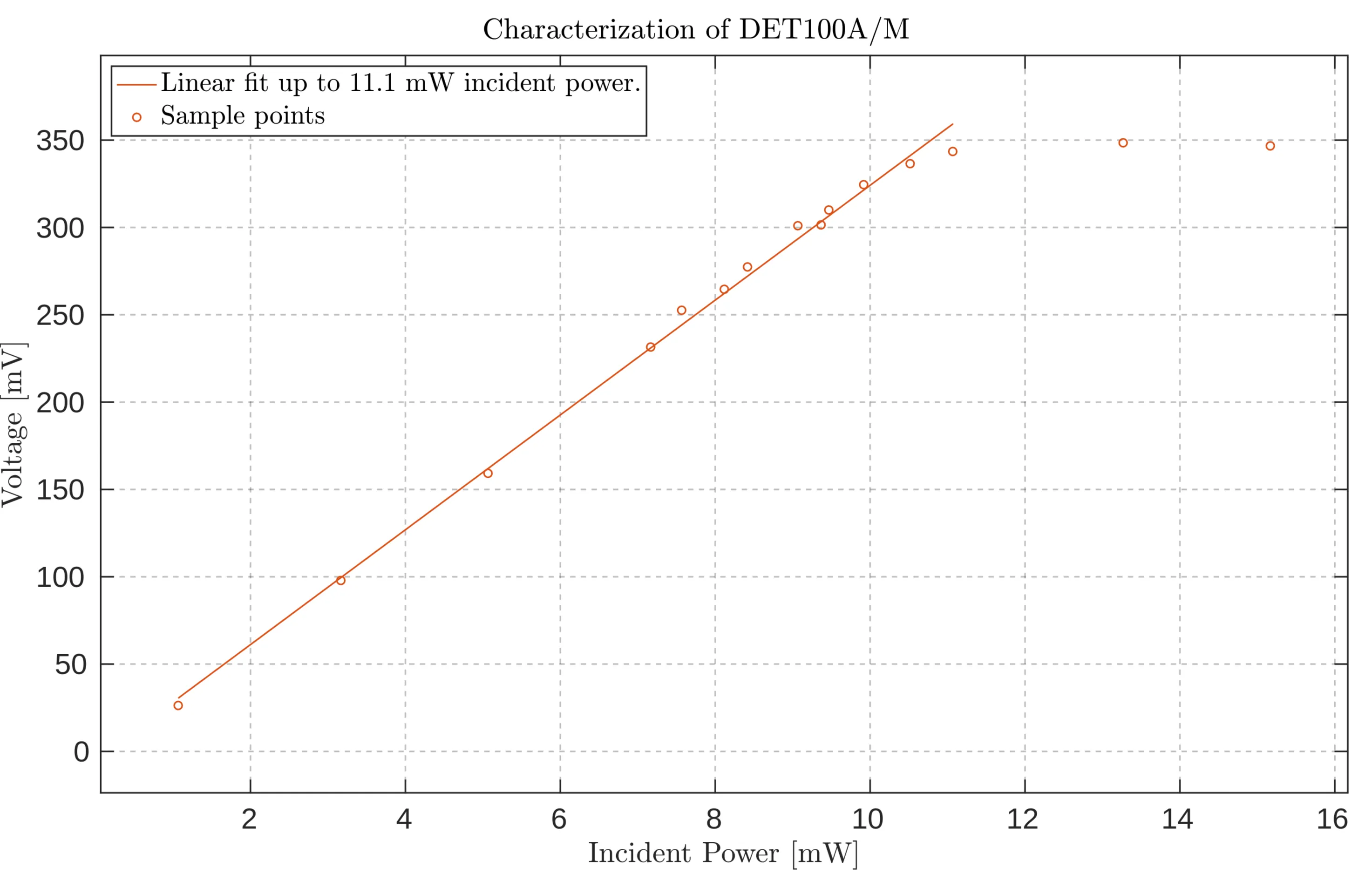
Characterisation of the silicon photodiode DET100A/M, showing a linear response for chosen points up to
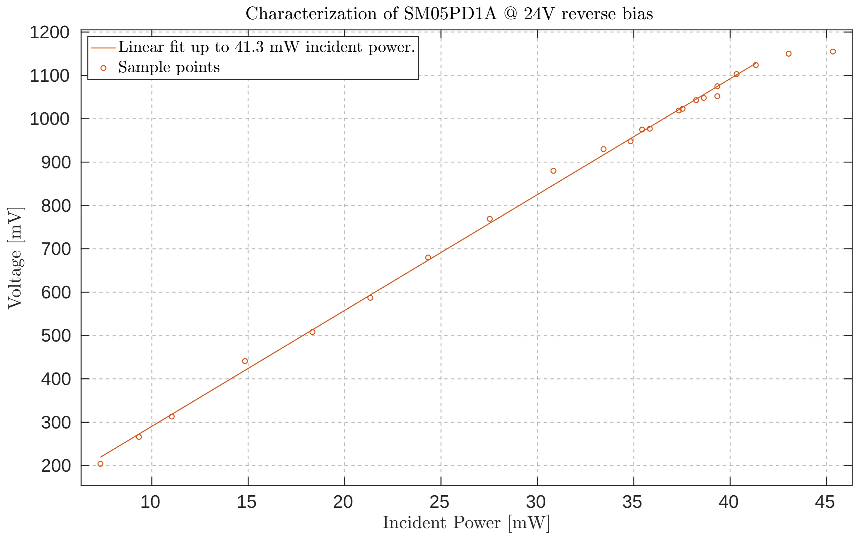
Characterisation of the silicon photodiode FDS100, showing a linear response for chosen points up to
These results suggest that the small-area FDS100 photodiode should enable the measurement of lower shot-noise levels. The shot-noise limit, expressed in units of
where
Therefore, in theory, the FDS100 photodiode should allow for the measurement of lower shot-noise levels. However, the results obtained did not align with expectations, as shown in the next two figures:
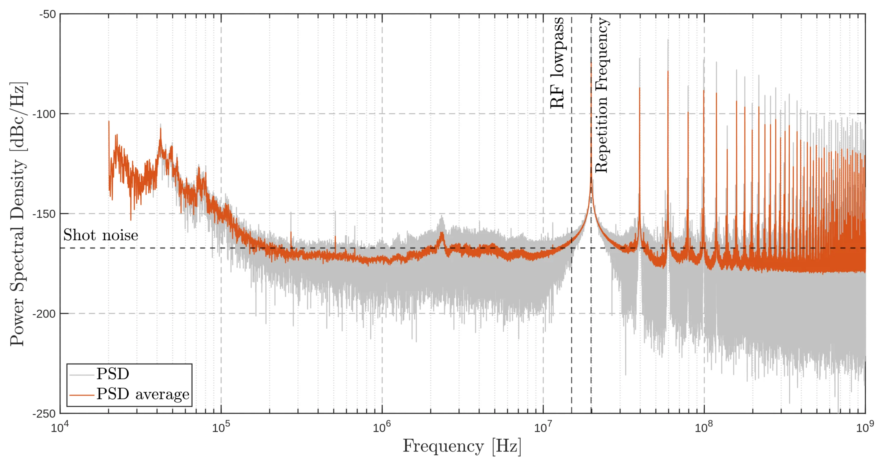
Noise PSD measured with the FDS100 photodiode at
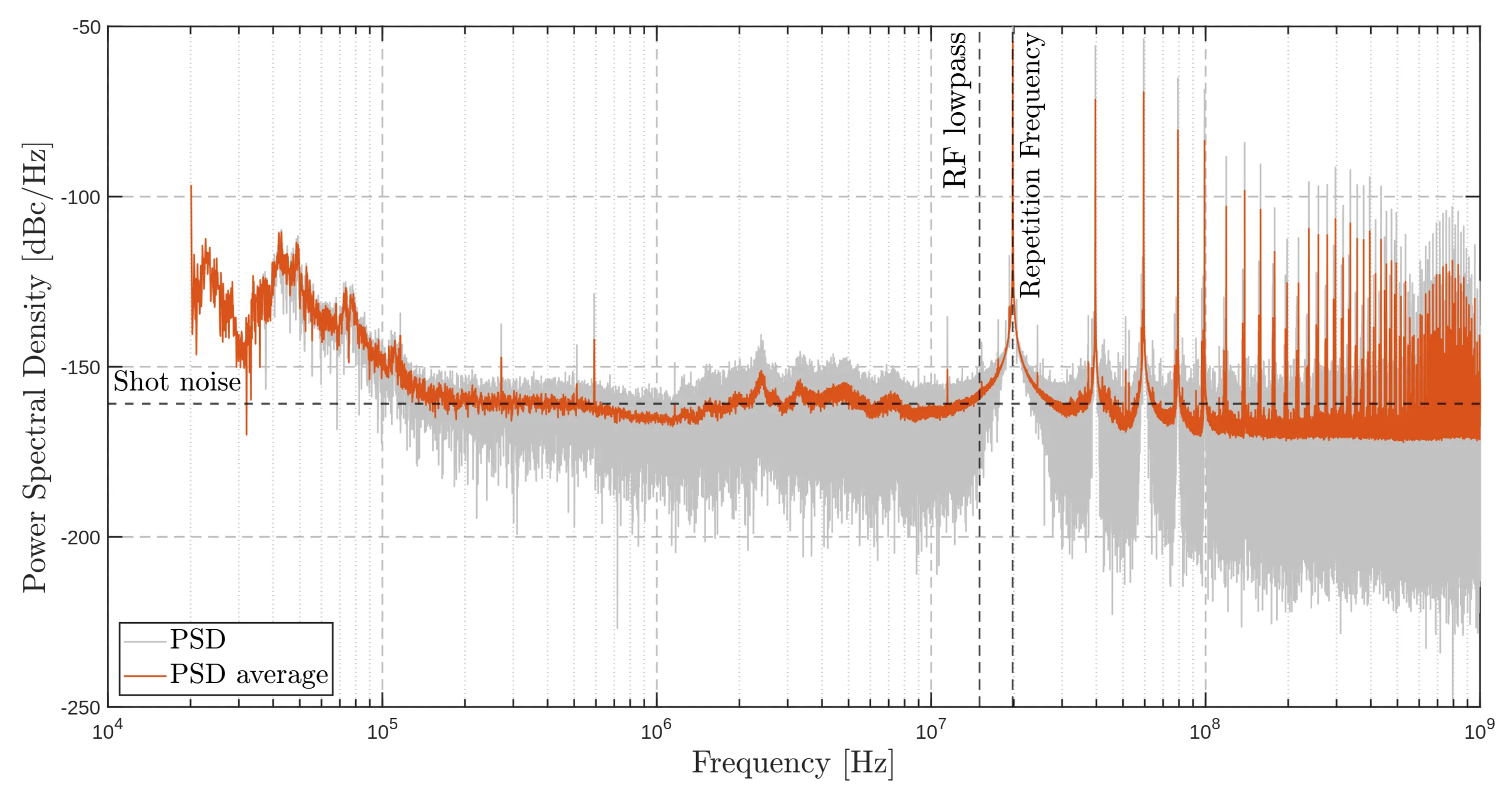
Noise PSD measured with the FDS100 photodiode at
As a result, the final noise measurements were carried out using the DET100A/M photodiode. The choice of photodiode plays a crucial role in determining the optimal measurement settings. With the appropriate photodiode selected, it is essential to ensure the measurements are taken within the photodiode's linear range, avoiding saturation. Saturating the photodiode can result in an artificially reduced shot-noise level, compromising the accuracy of the measurement results.
3.5.2 Noise Characterisation
Before delving into noise characterisation, it is essential to differentiate between the various types of laser noise when measuring with an oscilloscope: shot noise, amplifier noise, and oscilloscope (or quantisation) noise. Amplifier noise includes contributions from thermal (Johnson) noise and the amplifier's noise figure, increasing with the amplifier's gain and temperature. The noise power of the amplifier can be estimated as:
where
The next step involved performing the noise measurements using the selected photodiodes. The RIN spectrum of solid-state lasers typically exhibits much higher noise levels at low frequencies compared to the shot-noise limit at higher frequencies, so it is difficult to analyse the entire spectrum with a single, sensitive measurement. To overcome this, the RIN was measured separately in both the low- and high-frequency regions, each using different amplifiers optimised for their respective frequency ranges. For the low-frequency part, a
On the other hand, the oscilloscope allowed the use of a
Low-Frequency Region
For the frequency range from
To convert the signal from voltage to
where the factor of
which, like the carrier PSD, is expressed in units of volts squared. The spectral noise density is then calculated as:
High-Frequency Region
For frequencies above
When calculating the carrier spectral density in this region, the actual gain of the voltage amplifier must be considered. Although the DUPVA 1-70 was expected to deliver a
To obtain a meaningful shot-noise level, the DC voltage measured with this voltage amplifier is used. The shot-noise level can be determined using:
where
3.5.3 Optimising Sampling Rate for Accurate Noise Measurement
To conduct a meaningful noise measurement, a crucial factor to consider is the sampling rate of the measuring device - in this case, Teledyne Lecroy's WavePro 254 HD oscilloscope, which supports up to
To clarify this, it is useful to state the theorem more precisely in Shannon's original form:
The Nyquist-Shannon Sampling Theorem states: If a signal
Thus, assuming that there is no significant information above a few megahertz could be problematic. Aliasing can cause noise from higher frequencies to be sampled in a way that it appears at lower frequencies, potentially interfering with the measurements at frequencies of interest. This is why merely selecting a low sampling rate may not be sufficient; careful consideration of the highest frequencies present in the signal is essential to avoid misinterpreting the noise characteristics.
The careful reader might also wonder why the highest available sampling rate was not used. There are practical constraints, such as the maximum data file size and the speed at which the data can be processed. The oscilloscope allows for saving up to
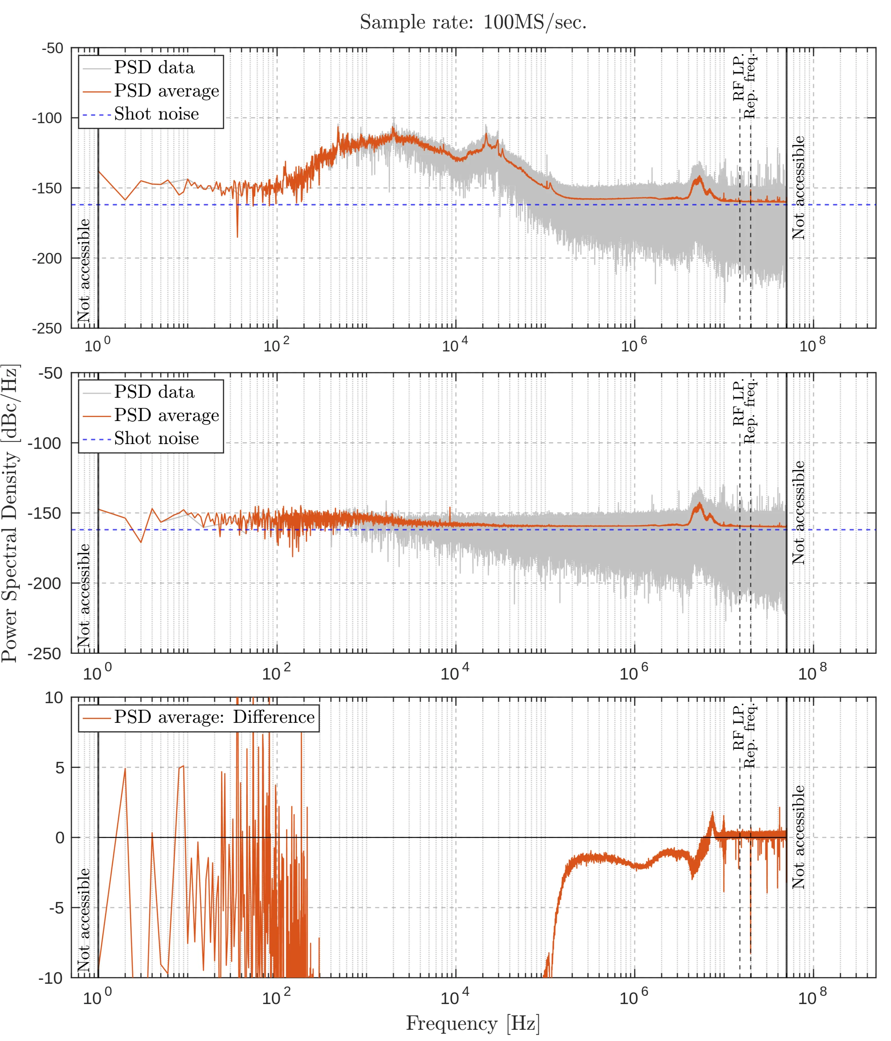
A series of experiments were conducted to determine the optimal sampling rate for measuring the noise spectral density of the laser. Noise measurements were compared under two conditions: a) with the laser light input and b) with the laser light blocked. The next five images display these comparisons, each consisting of three subplots: the top subplot shows the noise spectral density with the laser light input, with the raw Fourier transform in grey and the averaged trace in orange. The middle subplot shows the noise measurement with the beam blocked, again in raw (grey) and averaged (orange) traces. The bottom subplot presents the difference between the raw traces (grey) and the averaged traces (orange), with a black horizontal line indicating the zero mark.
Sample rate:
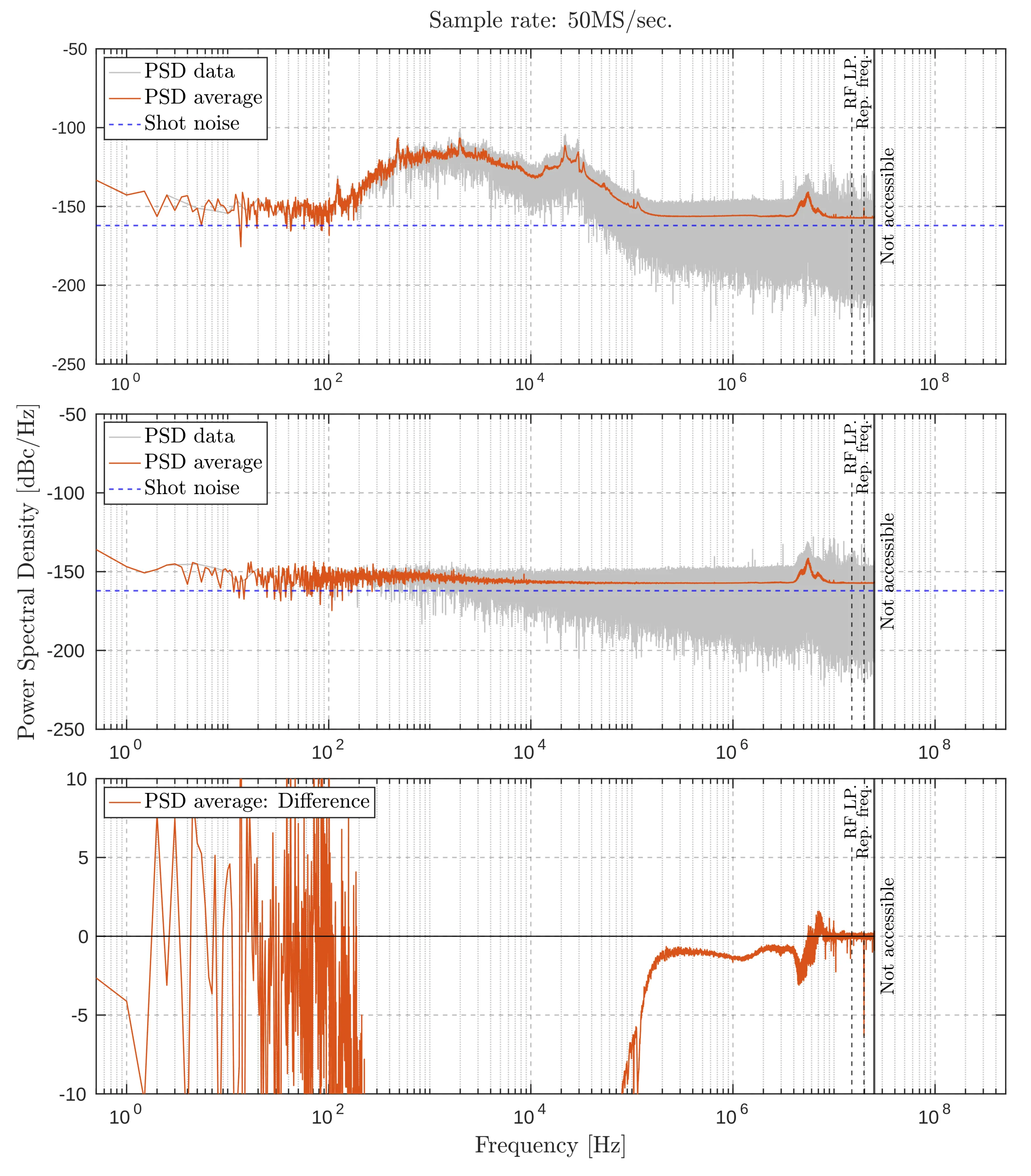
Noise measurement comparisons at a sampling rate of
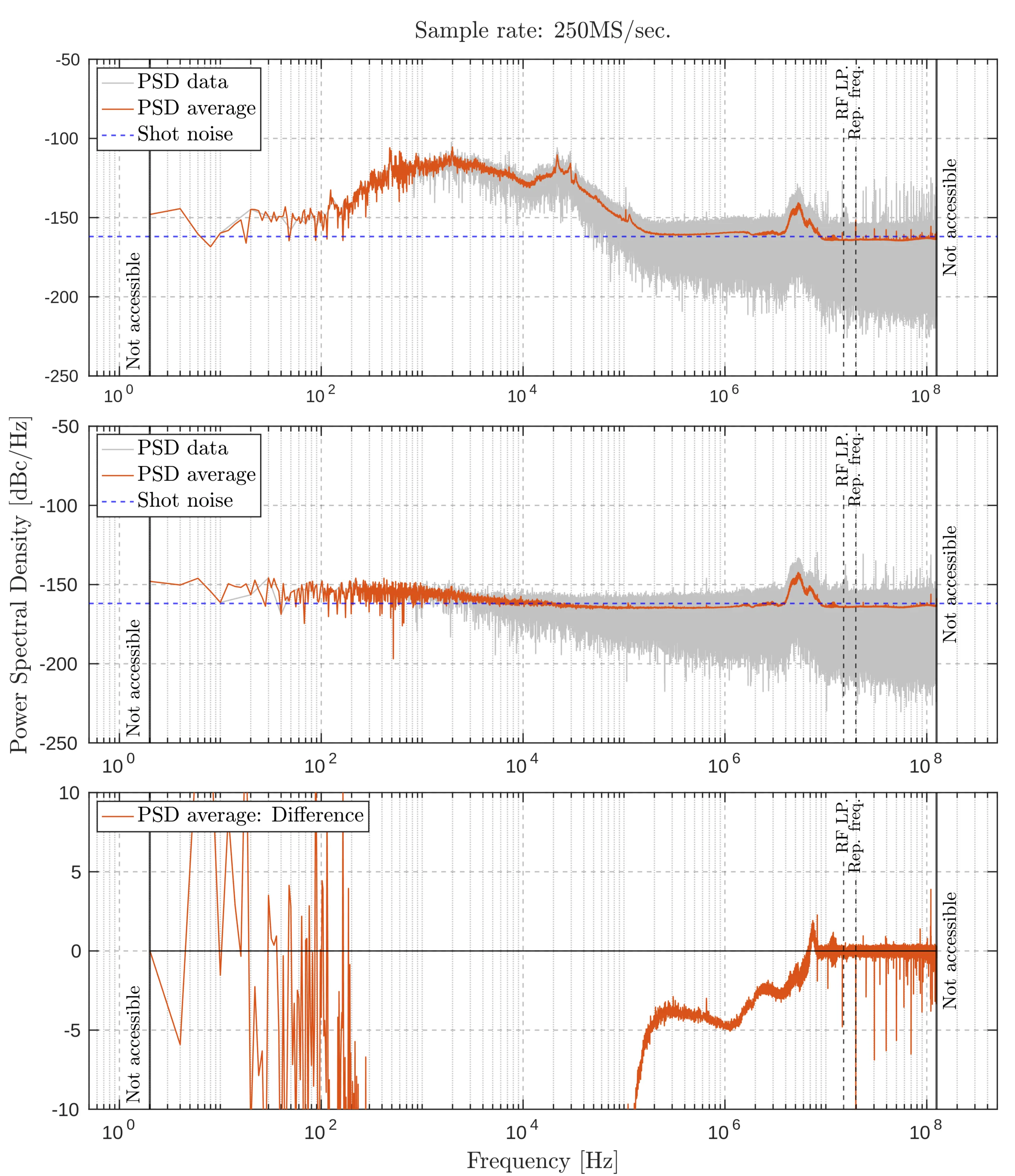
Sample rate:
Noise measurement comparisons at a sampling rate of
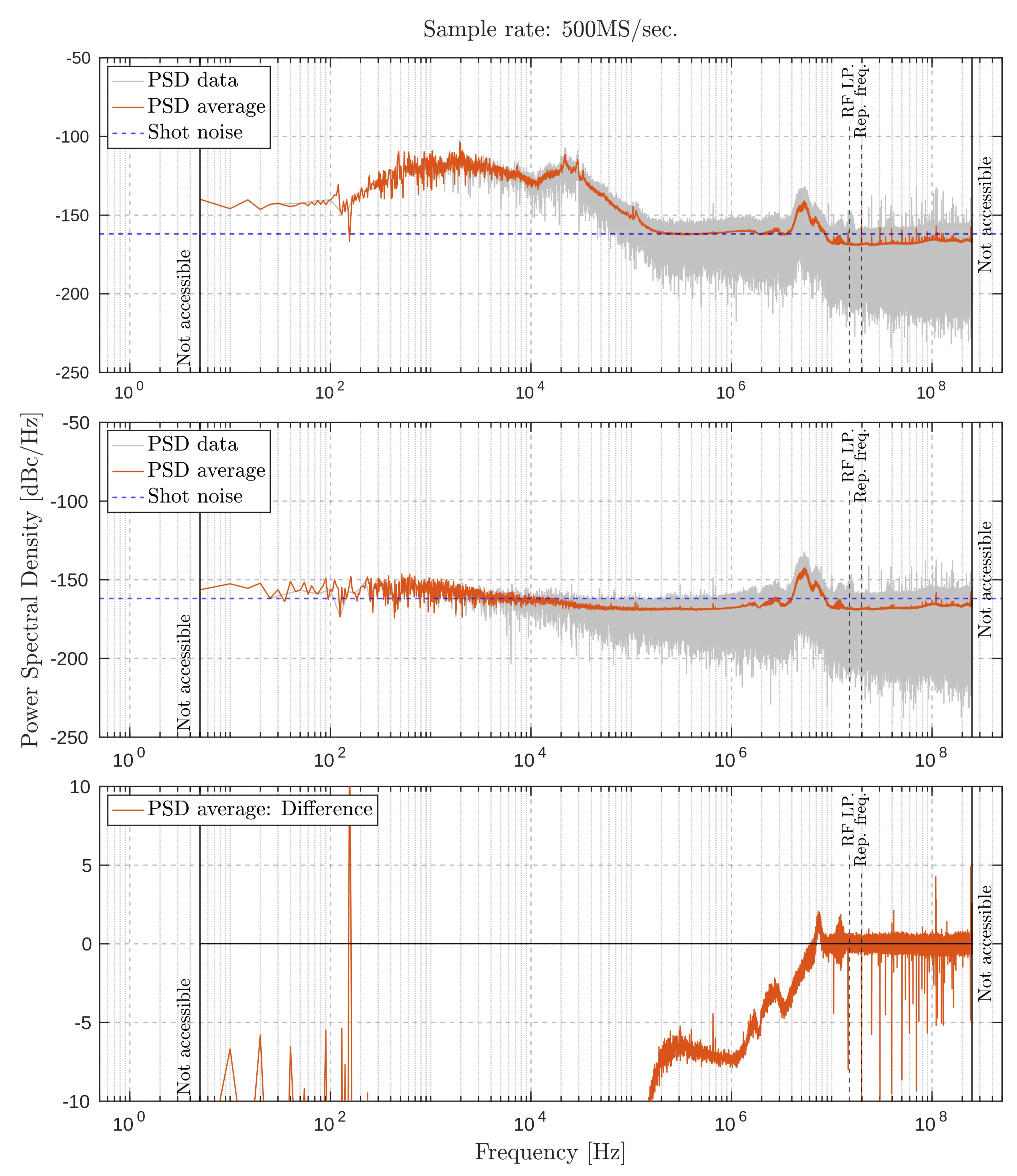
Sample rate:
Noise measurement comparisons at a sampling rate of
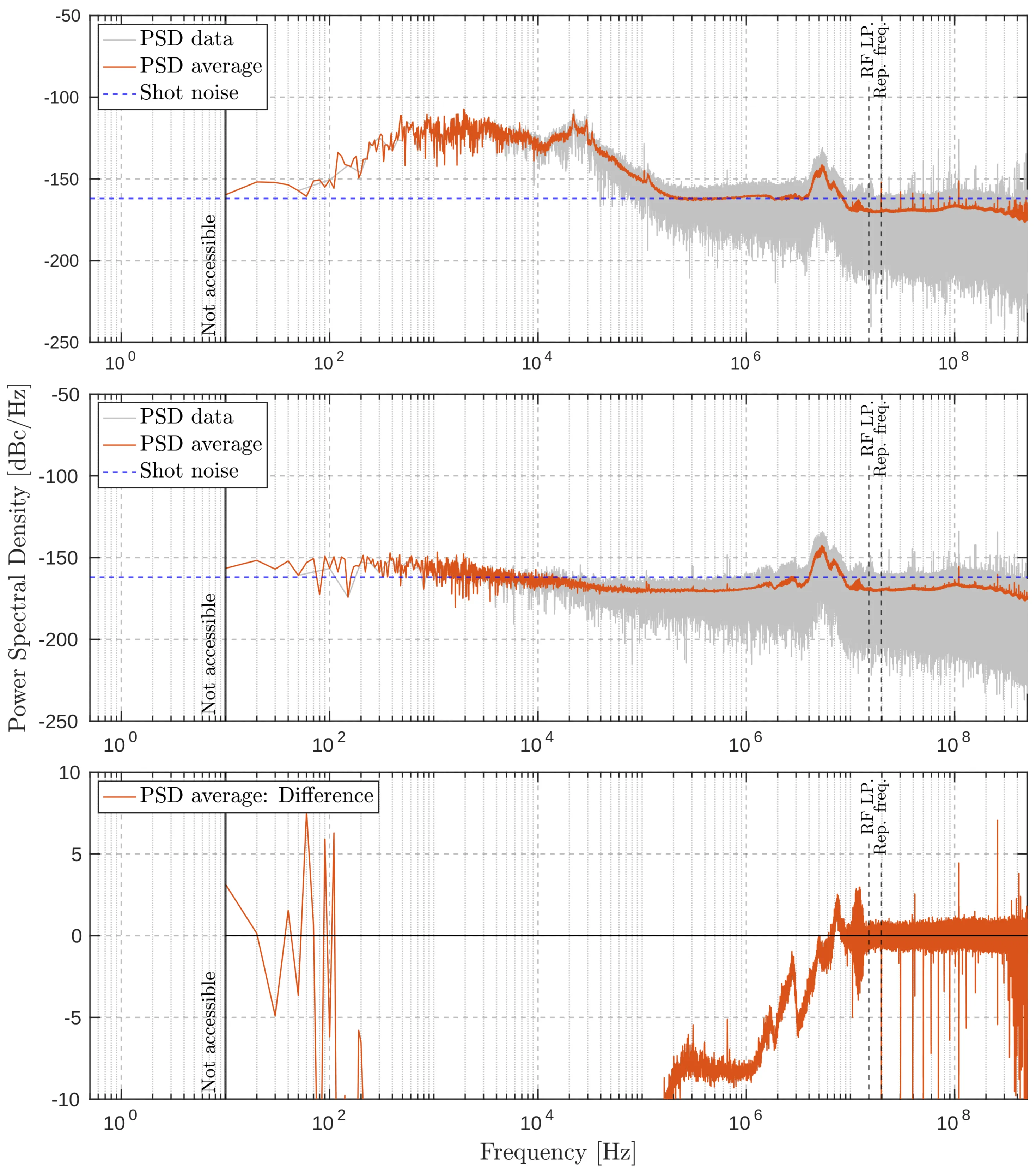
Sample rate:
Noise measurement comparisons at a sampling rate of : Top subplot shows the laser light input; middle subplot shows the blocked beam; bottom subplot displays the difference between raw and averaged traces. Aliasing effects are further reduced at this sampling rate, though larger data size may limit measurement duration.
Sample rate
Noise measurement comparisons at a sampling rate of
The results indicate that a sampling rate of
Note that each trace consists of exactly
Because the x-axis is kept constant, the lowest possible frequency component is determined by the
Resulting Noise Measurement
A good noise measurement can be conducted based on the preceding discussions and the collected data. Two traces were measured, one for each amplifier, and they overlapped in the frequency range from
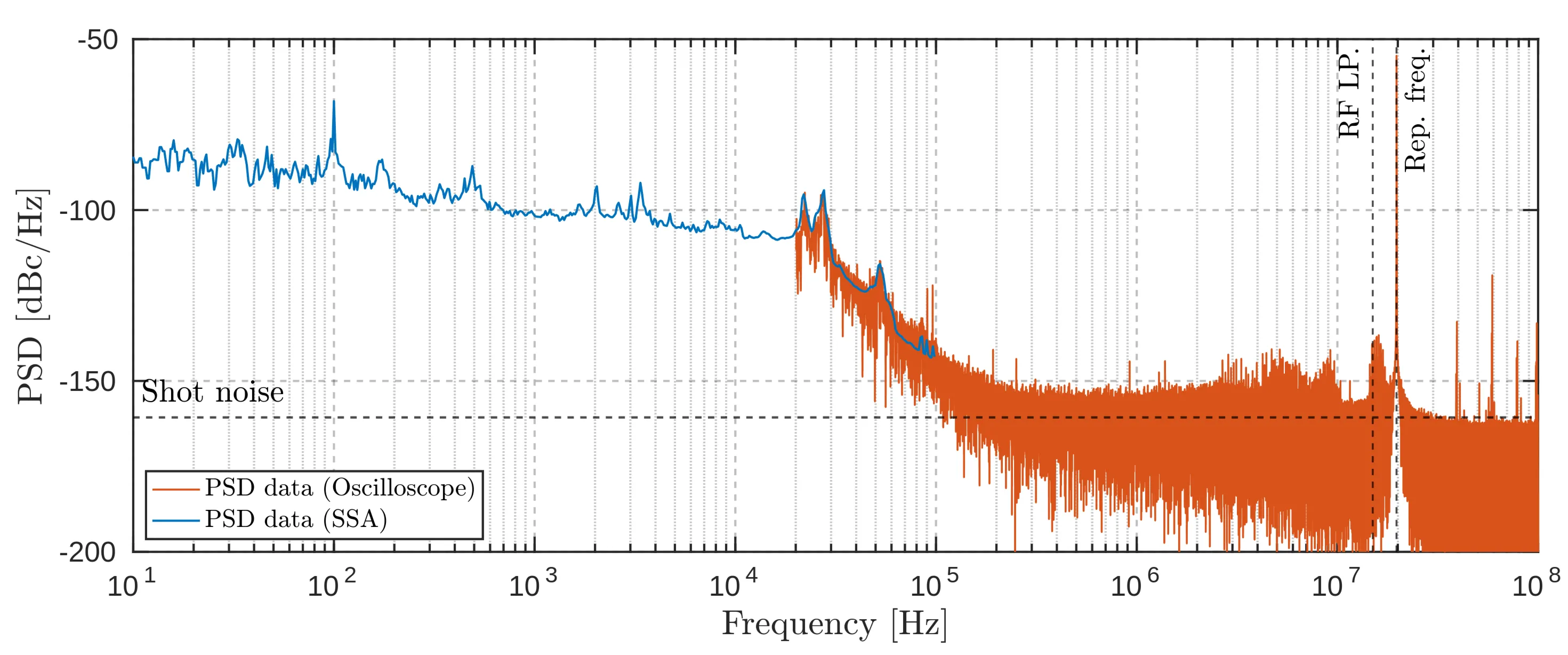
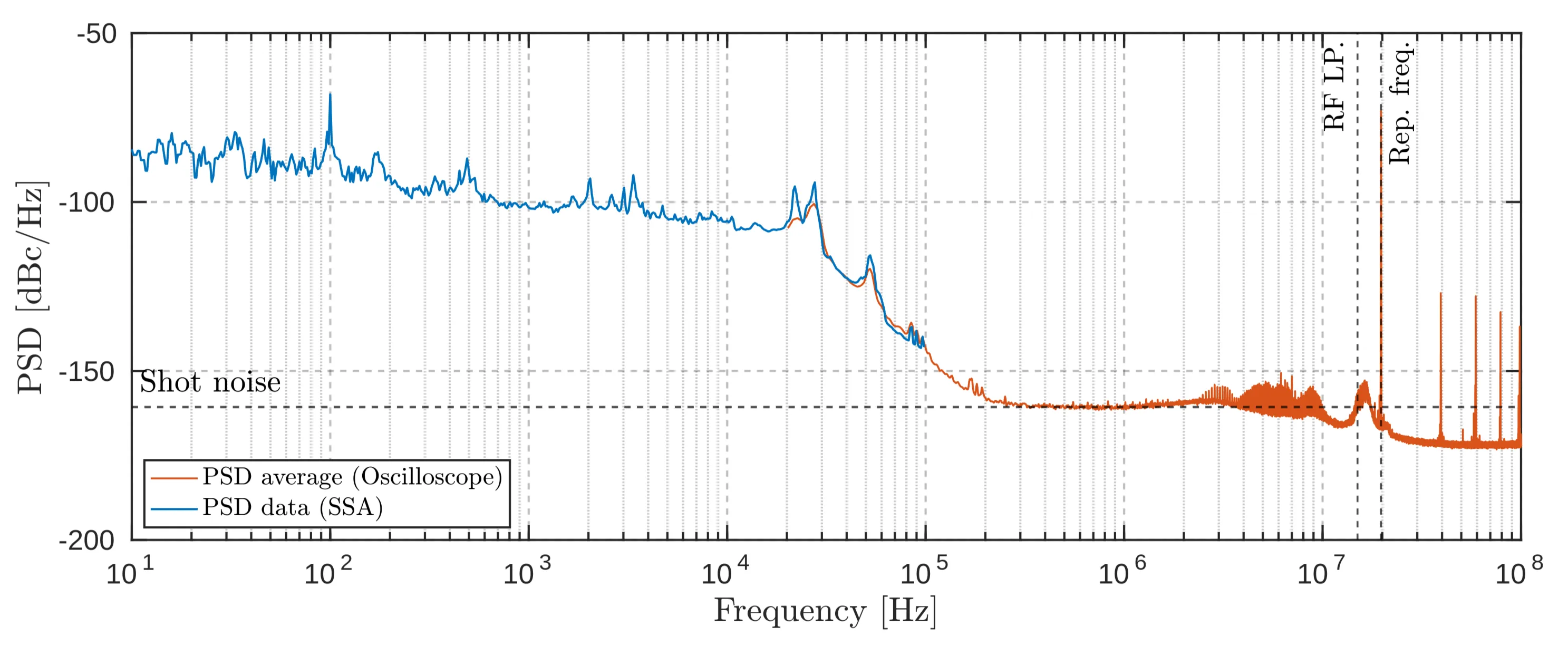
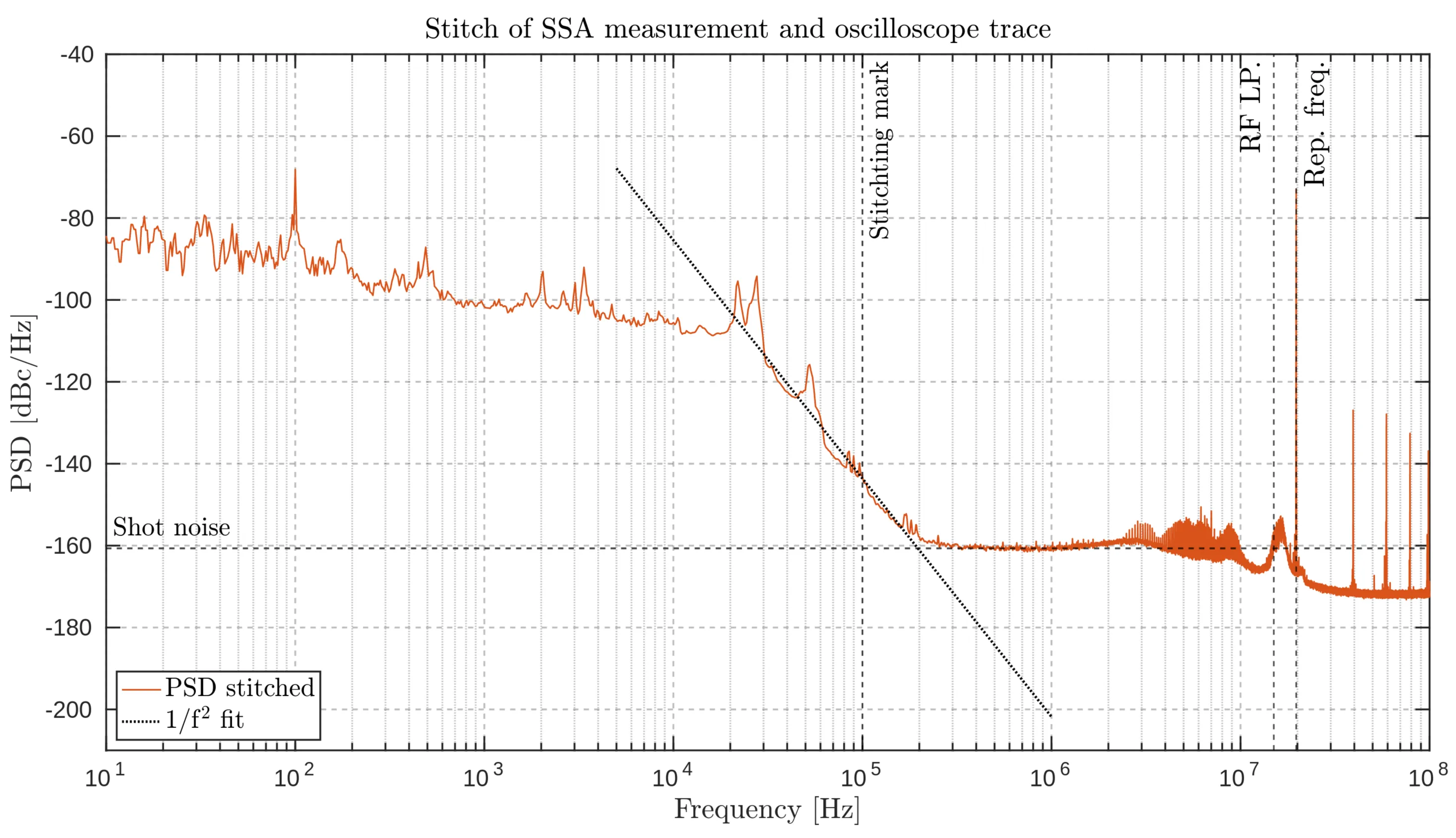
The blue trace is the noise PSD obtained from the SSA measurement, and the orange trace is the noise PSD obtained with the oscilloscope. As the oscilloscope operates with a finite sampling rate and measures for a finite time, it is unsurprising that the data appears very noisy. Therefore, it is impossible to draw any conclusions yet. To obtain visual clarity, the data has to be smoothed. This is done using Welch's method, as explained in the appendix. The resulting smoothed curve is depicted in the next figure, and now it can be seen that the noise curve runs into the shot-noise limit of
The stitching point is chosen as
3.6 Technical Considerations
In this section, technical considerations are addressed, and while not directly related to the core research, they are crucial for successful experimentation. These practical aspects can often become sources of frustration in the lab, as they are necessary but can be more challenging than anticipated. By sharing these insights, I hope to shed light on some of the unexpected daily challenges that can arise and potentially delay progress in the project.
As previously mentioned, most of the laser's power will be directed into a hollow-core photonic crystal fibre (HCPCF), where the spectral broadening will occur. Given that this power is approximately
The HCPCF is integrated with GLOphotonic's Powerlink system, which offers a comprehensive solution allowing for pressures up to
3.6.1.1 Beam Stabilisation
An active laser beam stabilisation system from MRC is employed to achieve the required precision, utilizing a combination of two 4QD detectors and two controllable mirrors, referred to as actuators. The next figure illustrates the setup schematically.
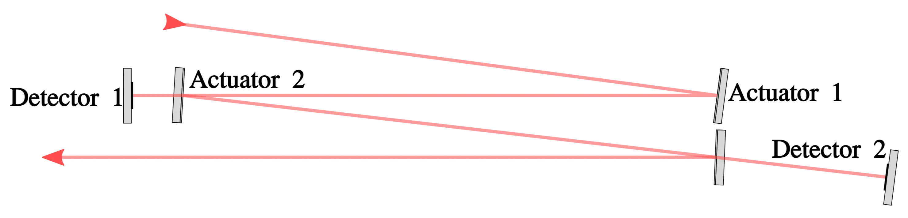
Schematic of the beam stabilisation setup. The system utilises two 4QD detectors and two actuators to stabilise the laser beam actively. Detector 1 receives input from the leakage of actuator 2, while detector 2 receives input from a subsequent mirror. The detectors continuously adjust the actuators to maintain the beam's position, compensating for any fluctuations in beam-pointing and ensuring precise alignment.
After being reflected by actuator 1, the laser beam reaches actuator 2, which then reflects it to the subsequent mirror. The movement of actuator 1 is controlled by detector 1, which receives input from the leakage of the mirror in front of actuator 2. Both detectors adjust their corresponding actuators to ensure the signal remains centred on their four photodiodes. This configuration compensates for beam-pointing fluctuations, thereby minimising variations in beam position and angle.
To verify the effectiveness of the stabilisation system, the fluctuations in beam position were compared with the stabilisation system turned on and off. The next figure compares the unstabilised and stabilised horizontal and vertical positions.
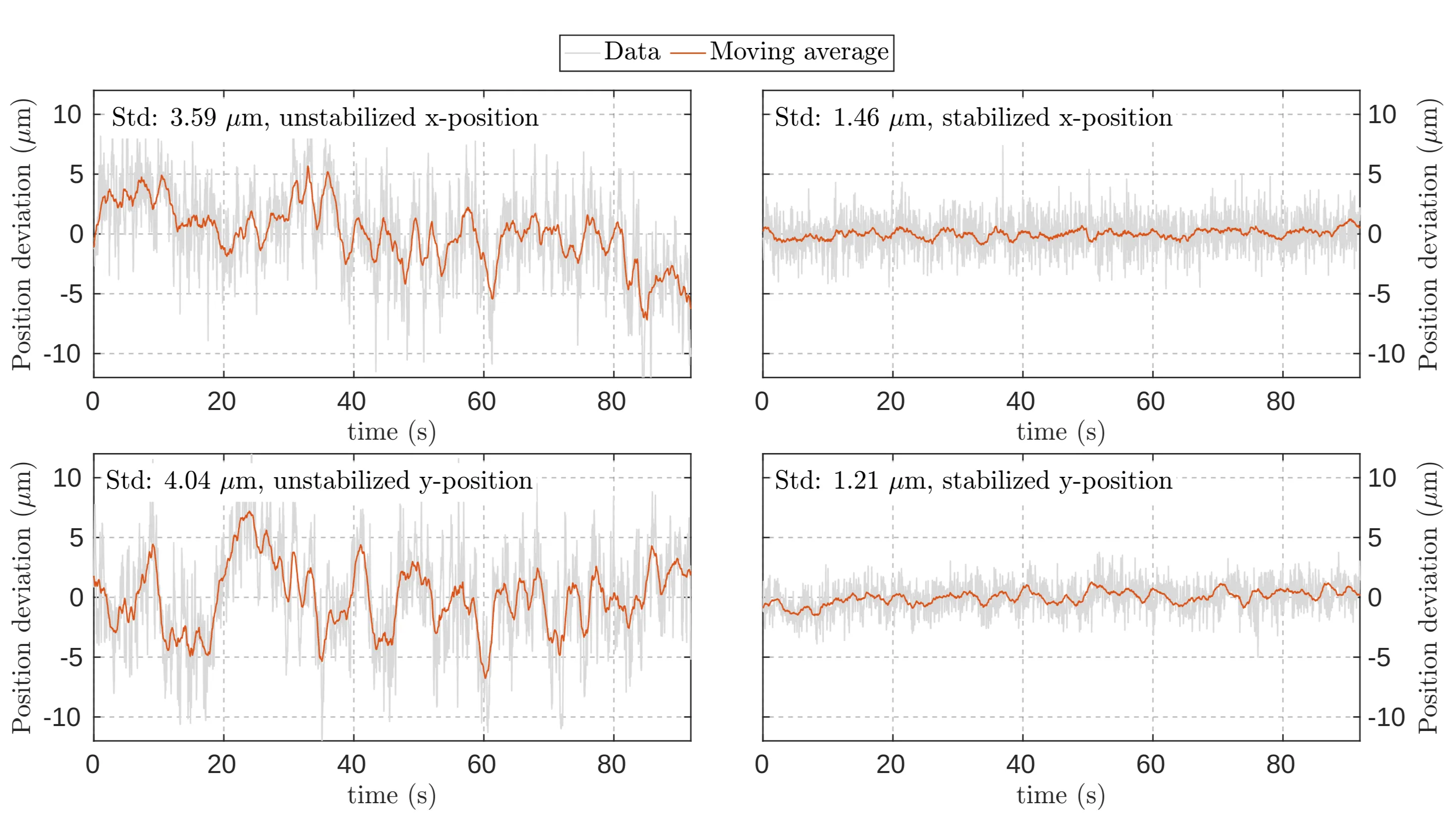
Comparison of beam position fluctuations in both
As shown, the beam stabilisation reduces the positional standard deviation from
3.6.1.2 Interlock: Pump Diode
When the active laser beam stabilisation system functions correctly, the laser beam couples into the fibre as intended. However, if there are significant drifts in the beam path, the beam position may move outside the working range of the actuators, rendering them unable to compensate for the misalignment. In such cases, the detectors may detect insufficient power, causing the actuators to default to a "zero position," which leads to the stabilisation system shutting down. If the beam is accidentally blocked or the control system loses power, the piezo motors drive the actuators to an extreme position. Both scenarios risk damaging the fibre and other optical components, making manual laser shutdown too slow to prevent potential damage. To address this, an interlock system has been implemented. Under normal operating conditions, the interlock circuit of the laser pump diode remains closed, allowing the pump laser to continue pumping the TDL gain medium. However, if any of the scenarios above occur, the circuit is opened, immediately stopping the pump diode and shutting down the laser. While this process is not instantaneous, it significantly reduces the risk of damage. The control system outputs a
However, in this configuration, the laser would never turn on because the beam stabilisation cannot function without an active laser, and the pump diode cannot be activated without beam stabilisation. To resolve this, a simple override switch was added to the system. The override temporarily bypasses the interlock, allowing the laser to turn on and the beam stabilisation to operate. Once the stabilisation is operational, the override switch is deactivated. The response time between the low TTL signal and the pump diode reaction is expected to be within the millisecond range, although it has not been explicitly measured. This interlock system provides the fastest safety mechanism to be implemented with relative ease and minimal complexity.
With this system in place, the only light that could potentially damage the fibre or other optical components after an error is detected is the residual light already oscillating within the cavity.
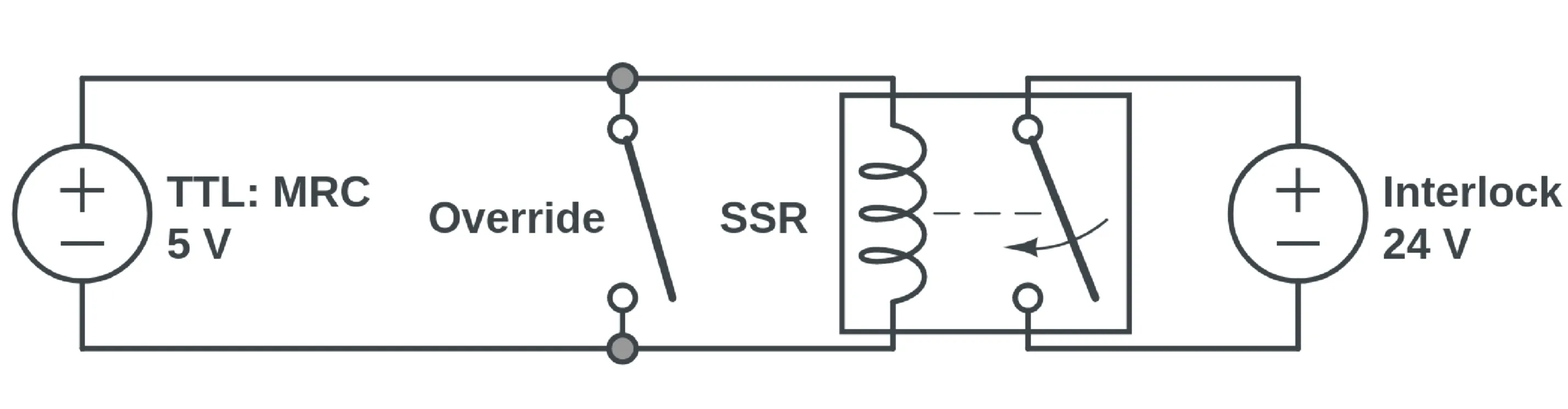
Electrical circuit of the pump diode interlock system, illustrating the components involved in safeguarding the laser setup. The circuit includes a
3.6.1.3 Interlock: Photodiode
After the light exits the fibre, it passes through a grating spectrometer, which allows for the selection of a specific wavelength range of the spectrum using a narrow slit. As shown in chapter 2.6.4, the power within a
3.7 Full Setup
The next figure provides a schematic overview of the experimental setup. This illustration includes key components such as active beam stabilisation, power and polarisation control, water cooling, and the grating spectrometer. The laser cavity, noise measurement, and diagnostic elements are represented schematically.
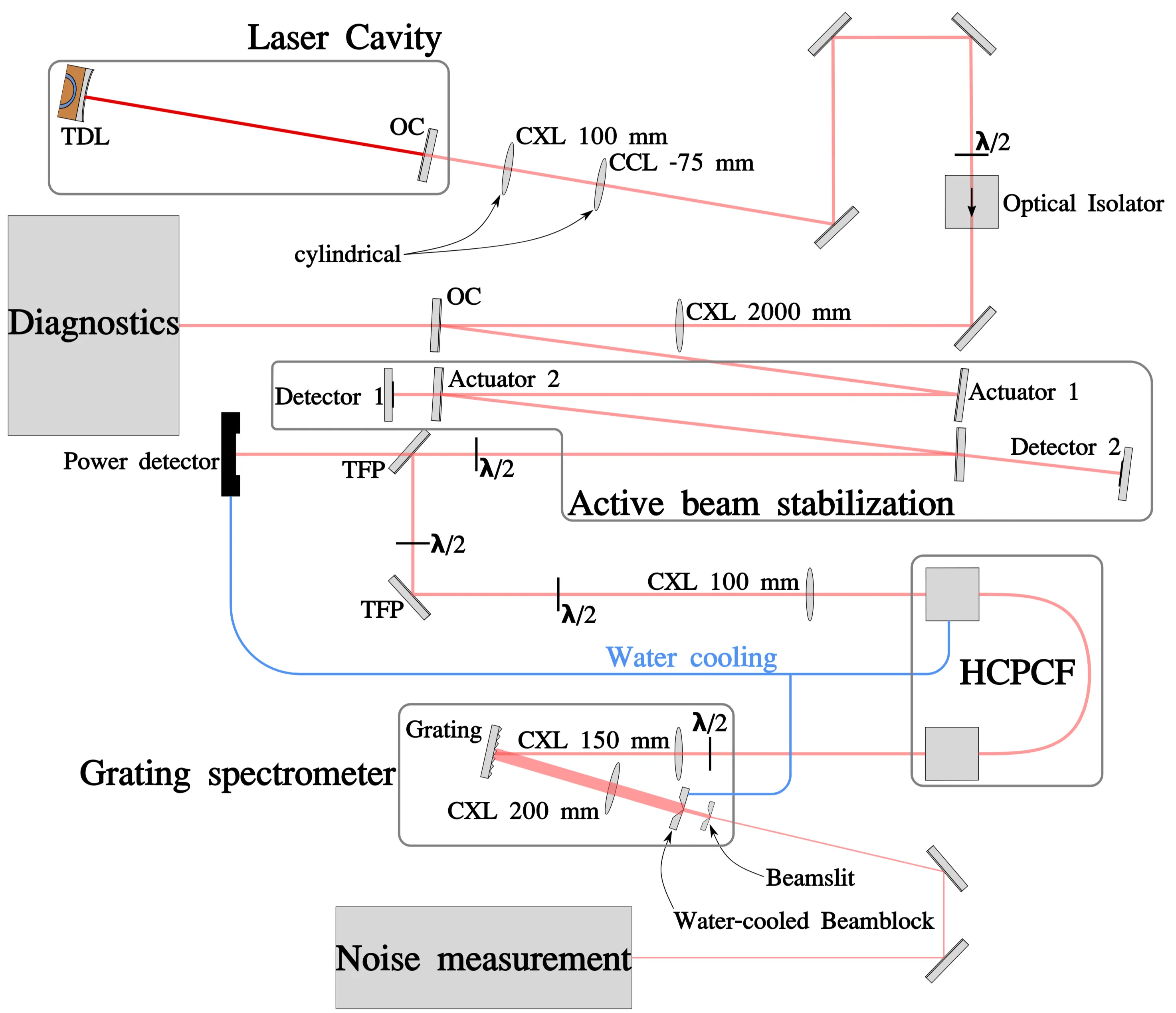
Schematic of the complete experimental setup, highlighting the active beam stabilisation, power and polarisation control, water cooling, and the grating spectrometer (distances not to scale). The laser cavity, noise measurement, and diagnostic components are shown schematically. CXL: convex lens, CCL: concave lens,
The next image shows the cavity as seen in the lab.
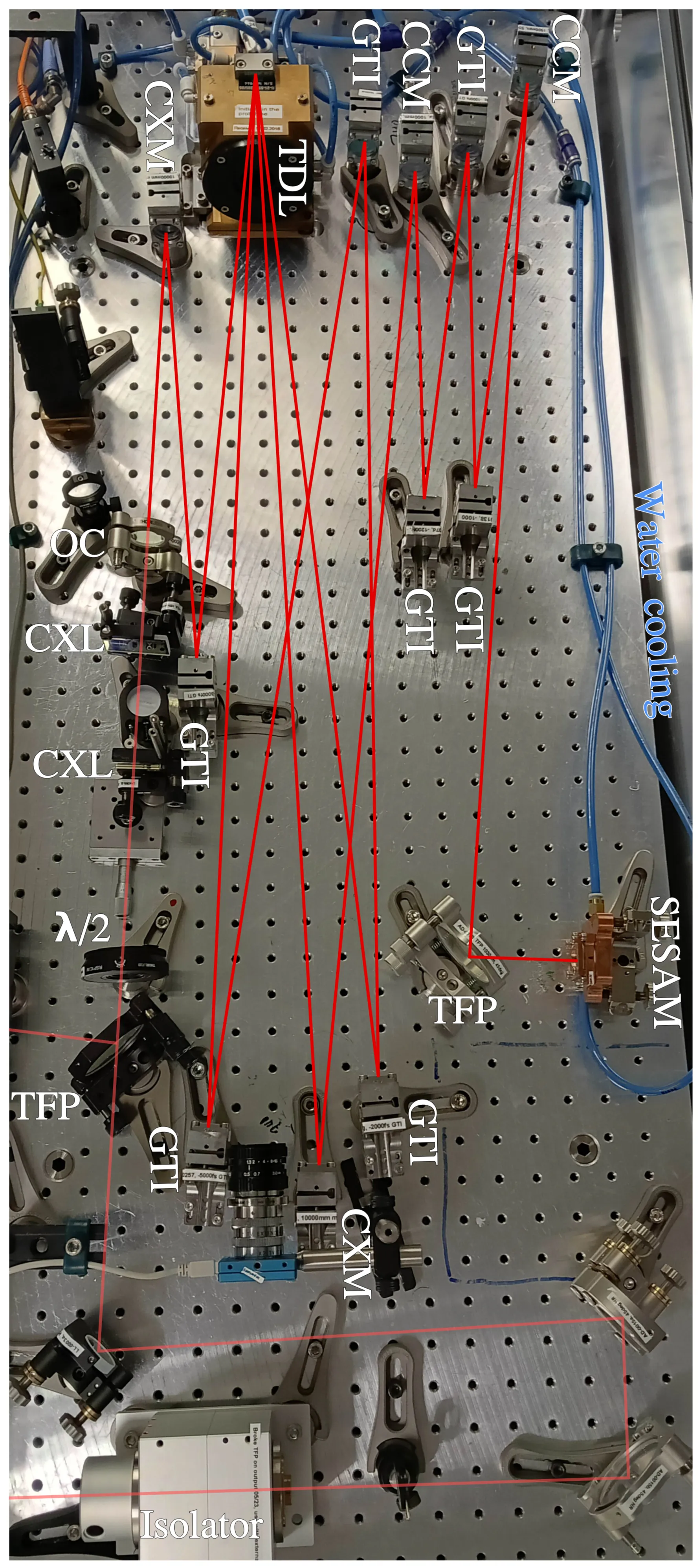
The final laser cavity as seen in the laboratory. The dark red path traces the laser light oscillating in the cavity, while the bright red shows the outcoupled light, indicating that the output power is