Jump back to chapter selection.

Table of Contents

2.1 Soliton modelocking
2.2 Saturable Absorbers and Passive Modelocking
2.3 Power Spectral Density, Relative Intensity Noise, and Signal-to-Noise Ratio
2.4 Noise of Modelocked Lasers
2.5 Shot Noise in Lasers
2.6 Influence of Spectral Broadening on Noise
2.7 Using Noise Gain from Spectral Broadening to Infer a Low Shot-Noise Level

2 Theory

2.1 Soliton modelocking

Soliton modelocking is a frequently used method to produce ultrashort pulses utilising the formation of solitons. When the effects of self-phase modulation (SPM) and negative group delay dispersion (GDD) balance, a soliton pulse is formed, which can propagate without pulse or spectral broadening in a dispersive medium. This balance is self-stabilising: since SPM depends on peak power while GDD does not, deviations in pulse parameters tend to be corrected, leading to a stable solution. This inherent stability makes solitons robust against distortions.

The starting point for any discussion on solitons is that they are the fundamental solution to the nonlinear Schrödinger equation (NLSE)

\frac{\partial}{\partial z} A (z, τ) = i \frac{k_{n}^{''}}{2} \frac{\partial^{2}}{\partial τ^{2}} A (z, τ) - i k n_{2} | A (z, τ) |^{2} A (z, τ)

where $k_{n}^{''} = \frac{\partial^{2} k_{n}}{\partial ω^{2}}$ is the second-order dispersion, and $τ = t - \frac{z}{v_{g}}$ is the retarded time with $v_{g} = \frac{\partial ω}{\partial k_{n}}$ the group velocity, which is generally frequency-dependent.

The fundamental soliton has the form

A_{S} (z, τ) = A_{0} \cdot sech (\frac{τ}{τ_{0}}) e^{- i ϕ_{0} (z)}

with $ϕ_{0} (z) = \frac{1}{2} k n_{2} I_{p} z$ being the nonlinear phase shift and $I_{p}$ the peak intensity. The characteristic pulse duration $τ_{0}$ is given by

τ_{0} = 2 \frac{| k_{n}^{''} |}{k n_{2} F_{p}},

where $F_{P}$ is the pulse fluence. The full-width-at-half-maximum (FWHM) pulse width, $τ_{p}$ , can then be obtained as $τ_{p} = 1.7627 τ_{0}$ . A soliton has a time-bandwidth product of $τ_{p} Δ ω_{p} = 0.3148$ with $Δ ω_{p}$ being the FWHM of the Fourier transform.

The following two figures compare the cases of negative and positive SPM, showing how positive GDD requires negative SPM to create a soliton.

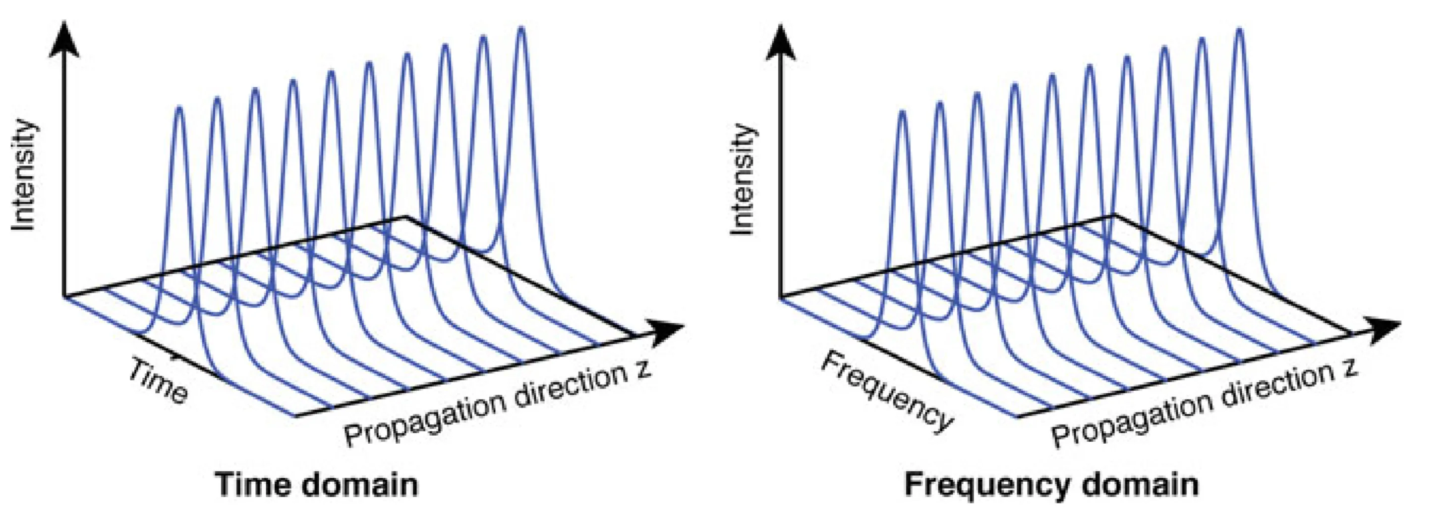
Attachments/Koeberlin_Master_Thesis.webp|700
A soliton can only form if the SPM has the opposite sign of the GDD. In this case, positive GDD requires negative SPM for a stable wavepacket (a soliton) to form. The shape remains unchanged in the time and frequency domain.

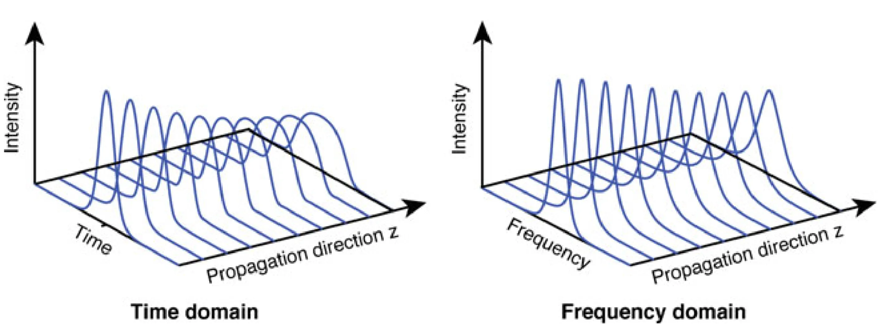
Attachments/Koeberlin_Master_Thesis 1.webp|700
Positive SPM amplifies the broadening effect of the already positive GDD. A soliton cannot form, and the pulse will keep broadening.

It is important to note that the preceding discussion assumes a uniform distribution of SPM and GDD. However, in practice, this uniformity is not always maintained within the laser cavity. Consequently, the pulse shape is only fully restored after a complete roundtrip through the cavity. During this roundtrip, the pulse may deviate from its ideal form, leading to temporary distortions.

2.1.1 Periodic Perturbations of Solitons

In lasers, solitons within the cavity are subjected to recurrent perturbations, such as those due to losses at the output coupler. Consider a soliton experiencing periodic perturbations within a system, represented by:

i ξ \sum_{m = - \infty}^{\infty} δ (z - m z_{a}) A (z, τ)

where $ξ ≪ 1$ is a small perturbation coefficient and $z_{a}$ is the periodicity of the perturbation. This model captures the essence of phenomena such as gain recovery in amplifiers or loss modulation in laser cavities.

From the nonlinear Schrödinger equation, incorporating the periodic perturbation gives:

\frac{\partial}{\partial z} A (z, τ) = i \frac{β_{2}}{2} \frac{\partial^{2}}{\partial τ^{2}} A (z, τ) - i γ | A (z, τ) |^{2} A (z, τ) + i ξ \sum_{m = - \infty}^{\infty} δ (z - m z_{a}) A (z, τ)

where $β_{2}$ is the group velocity dispersion (equivalent to $k_{n}^{″}$ ) and $γ$ is the nonlinear parameter (related to $k n_{2}$ ). For the analysis, we use the Ansatz:

A (z, τ) = A_{s} (z, τ) + u (z, τ)

where $A_{s} (z, τ)$ is the unperturbed soliton solution, and $u (z, τ)$ represents the perturbation. Substituting this into the NLSE and linearising, we obtain:

\frac{\partial}{\partial z} u (z, τ) \approx i \frac{β_{2}}{2} \frac{\partial^{2}}{\partial τ^{2}} u (z, τ) + i ξ \sum_{m = - \infty}^{\infty} δ (z - m z_{a}) A_{s} (z, τ)

Neglecting higher-order terms, the equation simplifies under the assumption $| u (z, τ) | ≪ | A_{s} (z, τ) |$ .

The periodicity introduces the possibility of resonance, where the perturbation frequency aligns with the natural frequencies of the system, potentially leading to significant growth in the amplitude of $u (z, τ)$ . This is the case if

m k_{a} = \frac{| k_{n}^{''} |}{2} (\frac{1}{τ_{0}^{2}} + ω_{m}^{2})

where $k_{a} = \frac{2 π}{z_{a}}$ and $τ_{0}$ is the characteristic soliton duration. To avoid such resonance, it is crucial that the perturbation period $z_{a}$ is much smaller than the soliton's characteristic length scale $z_{0}$ , ensuring:

z_{a} ≪ 8 z_{0}

Under this condition, the perturbation behaves almost as if it were continuous, allowing us to treat it with standard perturbation techniques.

2.2 Saturable Absorbers and Passive Modelocking

Until now, modelocking has been primarily explained through the nonlinear Schrödinger equation, highlighting the balancing effects of group delay dispersion and self-phase modulation. While the NLSE provides a powerful framework for understanding the formation and stability of soliton pulses, it does not fully capture all aspects of the laser dynamics. Specifically, the influence of gain, loss, and the initial pulse formation within the laser cavity are not addressed. In this section, passive modelocking is described from the perspective of saturable absorbers, such as the SESAM, with a particular focus on the formation of pulses.

The primary function of a saturable absorber (SA) is to implement self-amplitude modulation (SAM): it induces high losses for low-intensity light and low losses for high-intensity light. This results in loss modulation, as the pulse peak saturates the absorber more strongly than its wings. The starting point is the equation for the saturable loss coefficient:

\frac{d q}{d t} = - \frac{q (t) - q_{0}}{τ_{A}} - q (t) \frac{P (t)}{E_{sat, A}}

where $τ_{A}$ is the recovery time of the saturable absorber, indicating how long it takes for the losses to return to high values after the SA has been saturated, and $P (t)$ is the pulse shape. The SESAM used in this thesis has a recovery time of $9 ps$ , classifying it as a slow saturable absorber since $τ_{p} ≪ τ_{A}$ (where $τ_{p}$ is the pulse FWHM). This allows the neglect of recovery during the pulse duration. It can be shown that the saturable loss coefficient becomes

q (t) = q_{0} \exp (- \frac{E_{P}}{E_{sat, A}} \int_{0}^{t} d t^{'} f (t^{'}))

where $f (t)$ is a function normalised to 1 over the round-trip time. In this formulation, $q (t)$ is independent of the pulse length, and it can further be shown that the total loss of a pulse passing through the absorber is independent of the pulse shape:

q_{p} (E_{P}) = \int_{0}^{T_{R}} q (t) f (t) d t

In discussing passive modelocking, three cases are typically distinguished: (1) A slow saturable absorber with dynamic gain saturation, (2) a fast saturable absorber, or (3) a slow saturable absorber with no dynamic gain saturation. The last case is commonly referred to as soliton modelocking. The SESAM in this thesis operates in this regime as a slow, saturable absorber. To account for aspects such as gain and loss, the starting point is the Haus Master equation:

T_{R} \frac{\partial A (T, t)}{\partial T} = \sum Δ A_{i} = 0

which holds at steady-state over a "long" timescale $T$ , encompassing many round-trips. The linearised operators $Δ A_{i}$ represent changes due to gain, loss, and constant loss (such as output coupler losses). This description is valid for small changes per roundtrip, implying that the sum of changes balances out. By incorporating linearised operators for SPM and GDD, it is unsurprising that the solution to this equation is again a soliton pulse. However, the solution can be written in a slightly different form:

A (t) = A_{0} sech (\frac{t}{τ_{0}}) e^{i ϕ_{0} T / T_{R}} + continuum

Here, $τ_{0}$ is the characteristic soliton duration, and the continuum refers to a weak and temporally spread-out pulse, as depicted in the following figure:

Attachments/Koeberlin_Master_Thesis 2.webp|700
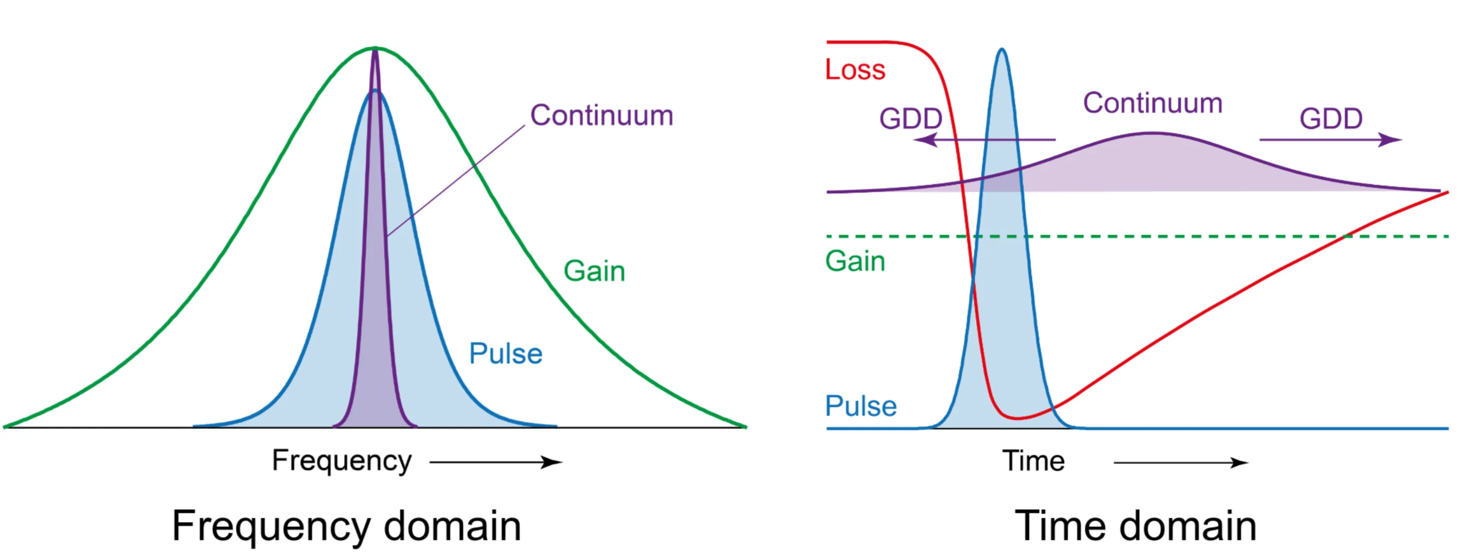
Illustration of soliton modelocking with gain and loss dynamics. The main soliton pulse (left) is stabilised by the interplay of gain and saturable absorption, while a weak, temporally spread-out continuum (right) is suppressed due to low intensity and the absence of self-phase modulation (SPM). The slow saturable absorber prevents the continuum from reaching the gain threshold, thereby maintaining a stable pulse within the laser cavity.

Due to its low intensity, the continuum does not experience SPM, resulting in its spread over time due to GDD (as shown on the right side of the previous figure). Because it is spectrally narrow, it experiences high gain. The slow SA is still fast enough to ensure that the continuum experiences enhanced losses, preventing it from reaching the threshold where gain equals losses. This stabilisation mechanism gradually removes the continuum or noise, thereby stabilising the soliton pulse. This explains how passive modelocking produces stable pulses despite the presence of the continuum. Passive modelocking ideally starts from noise fluctuations within the laser, where a noise spike is amplified more than other fluctuations until it reaches a steady state.

As mentioned, the SESAM used in this thesis is a slow, saturable absorber. The next figure depicts the reflectivity behaviour as a function of the incident fluence:

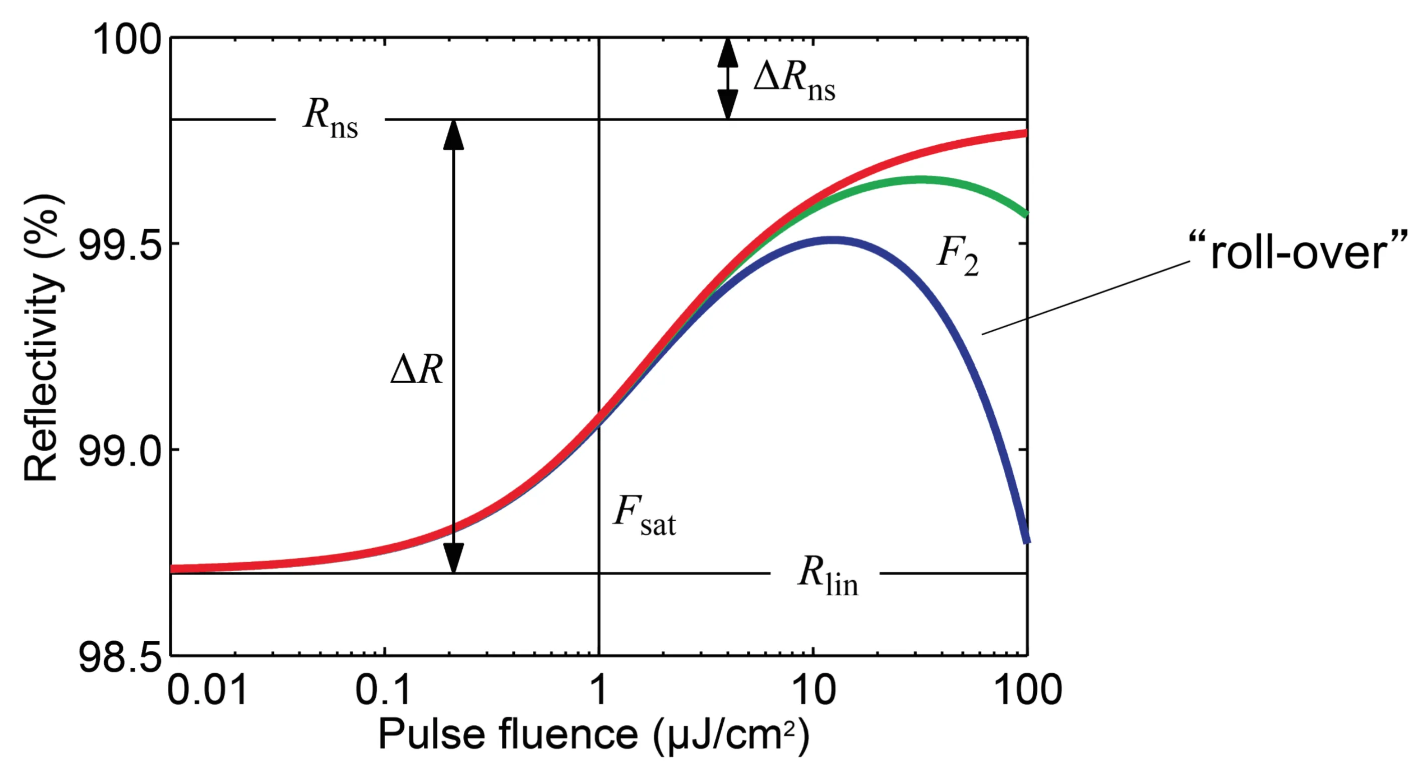
Attachments/Koeberlin_Master_Thesis 3.webp|700

As expected, the reflectivity initially increases with increasing fluence. However, eventually, the reflectivity decreases again due to second-order processes such as two-photon absorption. This leads to a rollover in the curve, typical of SESAMs, and is also called inverse saturable absorption.

2.3 Power Spectral Density, Relative Intensity Noise, and Signal-to-Noise Ratio

This section delves into several fundamental concepts essential to this thesis, including signal processing and optical communication: Power Spectral Density, Relative Intensity Noise, and Signal-to-Noise Ratio. To avoid confusion between various notations, this thesis adheres to the IEEE standard on random instabilities.

2.3.1 Power Spectral Density

The power spectral density (PSD) is a measure of the power content distributed across different frequencies within a signal. To illustrate, consider a general signal $x (t)$ , such as voltage as a function of time. We aim to understand how different frequencies contribute to its variance:

Var (x) = ⟨ x^{2} ⟩ - ⟨ x ⟩^{2}

In the context of digital signal processing, the energy $E$ of a continuous-time signal $x (t)$ is defined as

E = \int_{- \infty}^{\infty} | x (t) |^{2} d t

From Parseval's theorem, we further find that the energy in time is equal to the energy in frequency:

E = \int_{- \infty}^{\infty} | x (t) |^{2} d t = \int_{- \infty}^{\infty} | F (x) (f) |^{2} d f

where $F (x) (f)$ denotes the Fourier transform of $x (t)$ .
Therefore, power is simply energy divided by time:

P [x] = ⟨ x (t)^{2} ⟩

It is natural to define the energy spectral density as

E_{x} (f) = | F (x) (f) |^{2}

and consequently the (one-sided) power spectral density (PSD) for a stationary stochastic process $x (t)$ as

S_{x} (f) = lim_{T \to \infty} \frac{2}{T} ⟨ {| \int_{- T / 2}^{T / 2} x (t) e^{i 2 π f t} d t |}^{2} ⟩

The units of PSD are $[x]^{2} / Hz$ , implying power per unit bandwidth. Here, "power" does not necessarily refer to watts; for instance, in the context of voltage versus time, it denotes volts squared. Note that from now on, the PSD is always one-sided unless explicitly stated otherwise.

Another useful result comes from the Wiener-Khinchin theorem, stating that the power spectral density is the Fourier transform of the autocorrelation function $R_{x} (τ) = ⟨ x (t) x (t + τ) ⟩ :$

S_{x} (f) = 2 \int_{- \infty}^{\infty} R_{x} (τ) e^{- i 2 π f τ} d τ = 2 F (R_{x}) (f)

By applying the Wiener-Khinchin theorem, we can utilise autocorrelation measurements – often more straightforward to obtain experimentally – to derive the PSD. This is particularly useful in intensity noise measurements, where the autocorrelation function of the laser's intensity fluctuations is recorded over time. By transforming this autocorrelation data using the Wiener-Khinchin theorem, we can determine the PSD of the noise.

2.3.2 Relative Intensity Noise

Relative Intensity Noise (RIN) quantifies the intensity fluctuations of a signal relative to its mean intensity. For a signal $x (t) = \bar{x} + δ x (t)$ , where $δ x (t)$ represents fluctuations around the signal mean $\bar{x}$ , RIN is commonly defined as:

{RIN}_{x} (f) = \frac{2}{{\bar{x}}^{2}} \int_{- \infty}^{\infty} ⟨ δ x (t) δ x (t + τ) ⟩ e^{- i 2 π f τ} d τ = 2 \frac{F (R_{δ x}) (f)}{{\bar{x}}^{2}} = \frac{S_{δ x} (f)}{{\bar{x}}^{2}},

where the units are ${Hz}^{- 1}$ , and $S_{δ x} (f)$ refers to the Power Spectral Density of the fluctuations $δ x (t)$ .

The total PSD of the signal can be decomposed into the PSD of its mean and the PSD of its fluctuations:

S_{x} (f) = S_{\bar{x}} (f) + S_{δ x} (f),

where $S_{\bar{x}} (f)$ is the PSD of the mean. However, since the mean is constant, $S_{\bar{x}} (f) = 0$ for all non-zero frequencies (it is ${\bar{x}}^{2} δ (f)$ at $f = 0$ ). Thus, for practical purposes when considering AC-coupled noise ( $f \neq 0$ ), $S_{x} (f) \approx S_{δ x} (f)$ . RIN is often expressed in logarithmic units as "decibels relative to the carrier" (dBc/Hz), indicating how many decibels the noise is below the carrier level $\bar{x}$ .

2.3.3 Signal-to-Noise Ratio

The Signal-to-Noise Ratio (SNR) is a critical metric for evaluating the quality of a signal. It quantifies the ratio of the power of the signal to the power of background noise:

SNR = \frac{{\bar{x}}^{2}}{σ_{x}^{2} [f_{1}, f_{2}]},

where $σ_{x}^{2} [f_{1}, f_{2}]$ represents the variance of the signal's fluctuations, computed from the PSD across a specific frequency band $[f_{1}, f_{2}]$ . Here, the measurement duration typically sets the lower frequency limit $f_{1}$ , while the detection bandwidth determines the upper limit $f_{2}$ .

It is essential to specify these frequency limits because the variance, or root mean square (RMS) value, of the signal's fluctuations $\sqrt{σ_{x}^{2}}$ , is meaningful only within a defined frequency range. Therefore, defining the bandwidth is crucial for accurately assessing noise and, consequently, the SNR.

2.4 Noise of Modelocked Lasers

As this work primarily concerns noise, it is essential to discuss the noise characteristics of modelocked lasers. When light intensity $I (t)$ is detected by a photodetector, it ideally produces an electric current $J (t) \sim I (t)$ , and a spectrum analyser measures the power spectral density.

S_{I} (ω) \sim | I (ω) |^{2} = F (R_{I} (τ)) .

Therefore, the detector captures intensity noise originating from shot noise, Johnson (thermal) noise, and excess laser noise.

2.4.1 Noiseless Modelocked Laser Intensity

We begin with the intensity of an ideal, noiseless modelocked laser, which can be described by a delta-comb function:

I_{ideal} (t) = I_{0} T_{rep} \sum_{n} δ (t - n T_{rep}) ⟺ {\tilde{I}}_{ideal} (ω) = 2 π I_{0} \sum_{n} δ (ω - n ω_{rep}),

where $ω_{rep} = \frac{2 π}{T_{rep}}$ is the repetition frequency, $T_{rep}$ is the round-trip time, and $I_{0} T_{r e p}$ represents the energy of a single pulse. Consequently, the PSD for the ideal case becomes:

{\tilde{S}}_{ideal} (ω) = {(2 π I_{0})}^{2} \sum_{n} δ (ω - n ω_{rep}) .

2.4.1.1 Timing jitter

Any fluctuation in the optical path length results in timing jitter, as the repetition frequency is the inverse of the cavity round-trip time. Timing jitter $Δ T (t)$ can be mathematically described by:

δ (t - n T_{rep}) \to δ (t - n T_{rep} - Δ T (t)),

which shifts the temporal position of each comb line. This transforms the PSD of the ideal comb into:

{\tilde{S}}_{Δ T} (ω) = {(2 π I_{0} T_{rep})}^{2} \sum_{n} [δ (ω - n ω_{rep}) + {(\frac{n ω_{rep}}{2 π})}^{2} Δ T^{2} (ω - n ω_{rep})] .

The scaling goes as $\sim n^{2}$ , indicating that timing jitter increases more dramatically for higher harmonics. The standard deviation of timing jitter is then given by:

σ_{Δ T} = \sqrt{⟨ Δ T^{2} (t) ⟩} = \frac{1}{π} \sqrt{\int_{0}^{\infty} d ω {\tilde{S}}_{Δ T} (ω)}

When considering limits, we obtain:

σ_{Δ T} [f_{1}, f_{2}] = \frac{1}{π} \sqrt{2 \int_{f_{1}}^{f_{2}} d f \frac{P_{sb}^{(n)} (f)}{P_{c}^{(n)} (f)}}

where the index $s b$ stands for sideband and $c$ for carrier. The superscript $(n)$ denotes the $n$ -th harmonic. Due to the $n^{2}$ scaling, timing jitter has a more pronounced effect on higher harmonics, making them a crucial measurement point for accurately characterising the jitter in modelocked lasers. It is important to note that phase noise, which represents fluctuations in the phase of the comb lines, also contributes to timing jitter and is a key factor in determining the overall stability of the frequency comb.

2.4.1.2 Intensity noise

Normalised intensity noise is a significant type of noise in modelocked lasers. It is important to note that intensity noise and phase noise are often closely related, as the same underlying noise sources can induce both through coupling effects. Its effect changes the intensity as

I_{0} \to I_{0} (1 + N (t))

The corresponding PSD is:

{\tilde{S}}_{N} (ω) = {(2 π I_{0})}^{2} \sum_{n} [δ (ω - n ω_{rep}) + {\tilde{N}}^{2} (ω - n ω_{rep})]

which, in contrast to timing jitter PSD, is independent of the harmonic order $n$ . The standard deviation of intensity noise is:

σ_{N} = \sqrt{⟨ N^{2} (t) ⟩} = \frac{1}{π} \sqrt{\int_{0}^{\infty} d ω {\tilde{S}}_{N} (ω)}

However, it is crucial to note that calculating this standard deviation without specifying frequency boundaries is not just less meaningful; it is effectively meaningless. The standard deviation must always be provided with well-defined frequency limits for accurate and practical measurements. This ensures that the noise characteristics are appropriately quantified and relevant to the specific application or measurement scenario:

σ_{N} [f_{1}, f_{2}] = \sqrt{\frac{P_{sb} [f_{1}, f_{2}]}{P_{c}}}

where $P_{sb} [f_{1}, f_{2}]$ is the power from the integration over the noise sidebands within the specified frequency boundaries.

2.5 Shot Noise in Lasers

Shot noise is a fundamental type of noise in electronic and optical devices, arising from the discrete nature of charge carriers (electrons) and light (photons). In lasers, shot noise is a consequence of the quantum statistical nature of photon emission. Although photon emission in lasers primarily occurs through stimulated emission, which leads to correlated emission events, the underlying processes are inherently probabilistic. The random nature of these processes, which follow a Poisson distribution, results in intrinsic fluctuations in the number of photons detected over a given interval. These fluctuations are inherent to the light itself, regardless of the stability of the light source.

For a photodiode detecting light, the photocurrent $I (t)$ generated is proportional to the number of incident photons per unit of time. Assuming a constant average number of photons arriving per unit time, the resulting photocurrent will exhibit fluctuations due to the Poisson nature of photon arrival times. The root mean square (RMS) value of the shot noise current can be described by:

I_{shot} = \sqrt{2 e \bar{I} Δ f}

where $e$ is the elementary charge, $\bar{I}$ is the average photocurrent, and $Δ f$ is the bandwidth of the measurement system.

According to Schottky's theorem, the power spectral density (PSD) of shot noise in the photocurrent is given by:

S_{I, shot} = 2 e \bar{I}

which highlights the frequency independence of shot noise, classifying it as white noise. A derivation of this theorem is provided in the Appendix. The PSD of shot noise related to optical power fluctuations can also be expressed as:

S_{P, shot} = 2 ℏ ω \bar{P}

where $ℏ$ is the reduced Planck's constant, $ω$ is the angular frequency of the light, and $\bar{P}$ is the average optical power.

Using the definitions above, the Relative Intensity Noise for shot noise can be expressed as:

{RIN}_{shot} = \frac{2 e}{\bar{I}} or {RIN}_{shot} = \frac{2 ℏ ω}{\bar{P}}

From these results, we can deduce the following behaviour: Attenuating the laser output increases the relative intensity noise (RIN) due to shot noise. This is because reducing the power of a coherent beam makes quantum fluctuations more significant relative to the signal. Conversely, increasing the power reduces the relative impact of shot noise as the signal strength increases; however, this also increases the absolute level of shot noise due to the higher photon count. Additionally, increasing the bandwidth increases shot noise power, as more noise fluctuations are detected within the broader frequency range. Detector efficiency is also crucial: lower efficiency leads to fewer detected photons, which may reduce the absolute shot noise but increase the relative shot noise per detected signal, thereby degrading the signal-to-noise ratio.

While shot noise tends to dominate at high frequencies, the specific frequency at which this occurs can vary widely depending on the laser architecture, gain medium, and other factors. For instance, in solid-state lasers, shot noise may become significant at frequencies around $1 MHz$ or higher. In contrast, shot noise might dominate at much lower frequencies in other systems or may never become the dominant noise source, for instance, in fibre lasers.

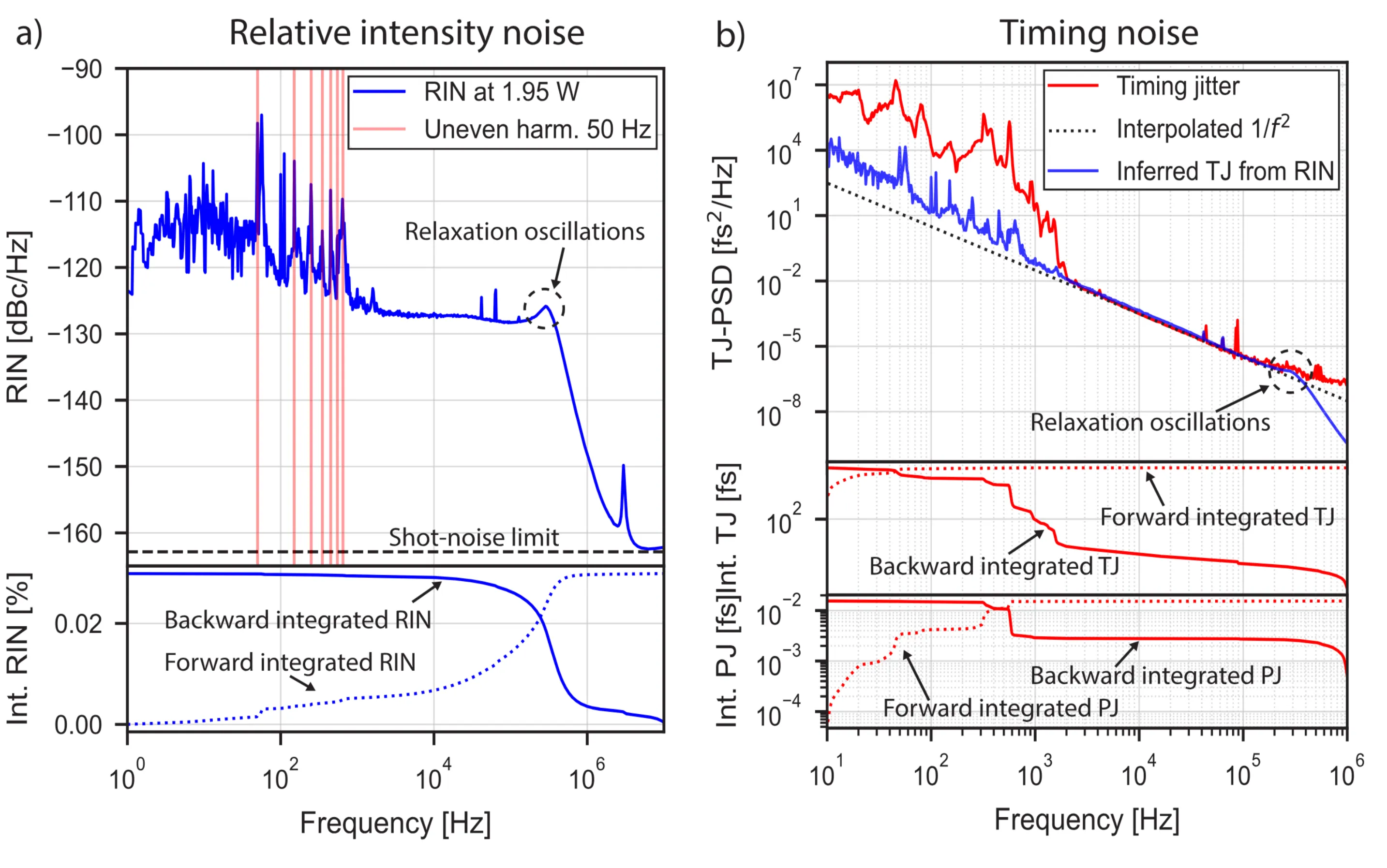
At lower frequencies, various other noise sources become significant, including relaxation oscillations, pump noise, thermal noise, and $1 / f$ noise. These sources contribute to the overall noise profile of the laser and can overshadow shot noise at these frequencies. To illustrate this effect, the next figure shows the RIN and timing noise of a SESAM modelocked Ytterbium-doped solid-state laser with a GHz repetition rate. Relaxation oscillations can clearly be seen as a prominent peak, whereas the laser noise approaches the shot noise limit at higher frequencies:

Attachments/Koeberlin_Master_Thesis 4.webp|700
Relative intensity noise (RIN) and timing noise characteristics of a SESAM modelocked Ytterbium-doped solid-state laser operating at a GHz repetition rate. The figure illustrates various noise sources, with relaxation oscillations appearing as a prominent peak at lower frequencies. At higher frequencies, the noise level approaches the shot noise limit, indicating the dominance of quantum noise in this region.

A detector is said to be "shot noise-limited" when the predominant noise source affecting its performance is shot noise rather than thermal or electronic noise. In such systems, improving the SNR primarily involves increasing the optical power, as shot noise power scales linearly with optical power, while the signal power scales quadratically with optical field or linearly with optical power, leading to SNR improvements. Achieving shot noise-limited performance is desirable in applications requiring high precision and sensitivity, such as quantum optics and spectroscopy.

2.6 Influence of Spectral Broadening on Noise

Spectral broadening is a significant nonlinear optical effect utilised in various applications, such as supercontinuum generation, pulse compression, and potentially in enhancing noise measurement techniques. During spectral broadening, noise is influenced. In the frequency range where shot noise is the dominant noise source of the unbroadened laser system, spectral broadening can cause an increase in the noise PSD.

This section explores the potential of using spectral broadening to influence noise, particularly emphasising the Kerr effect in high-pressure Xenon gas-filled hollow-core fibres. While not traditionally associated with noise measurement, this approach offers a novel perspective on how nonlinear effects can interact with and potentially manage different noise contributions in optical systems.

2.6.1 The Optical Kerr Effect

The optical Kerr effect causes the refractive index of a material to become intensity-dependent. To the first order, this can be expressed as:

n (I) = n + n_{2} I,

where $n_{2}$ is the nonlinear refractive index coefficient, typically of the order of $10^{- 16} {cm}^{2} / W$ for solids (equivalent to $10^{- 20} m^{2} / W$ ), making this effect observable only at high intensities. This leads to a nonlinear phase shift:

φ (t) = k_{0} n L + δ I (t)

with $δ = k_{0} n_{2} L$ being the self-phase modulation coefficient ( $k_{0}$ is the free-space wavevector). Consequently, the instantaneous frequency becomes non-zero:

ω (t) = \frac{d φ}{d t} = δ \frac{d I}{d t}

indicating that SPM broadens the bandwidth of a pulse. In the leading edge of the pulse, where $\frac{d I}{d t} > 0$ , lower frequencies are generated, and on the trailing edge, higher frequencies are produced. This phenomenon does not occur in linear optics and is intrinsic to nonlinear effects.

Various methods exist for spectral broadening, including the previously discussed self-phase modulation resulting from intensity-dependent phase shifts. Additionally, cross-phase modulation, four-wave mixing, Raman scattering, and supercontinuum generation are significant contributors to spectral broadening. Spectral broadening has applications in optical communication, metrology, and microscopy, among other fields.

2.6.2 Simulation

In the experiment, we utilise a high-power laser and high-pressure Xenon gas, chosen for its large nonlinear refractive index of $n_{2}^{(Xe)} = 8.1 \cdot 10^{- 23} m^{2} / W$ . This value is approximately six times larger than that of air or the noble gas Argon, both at $n_{2}^{(Ar, Air)} = 1.4 \cdot 10^{- 23} m^{2} / W$ . Additionally, since the nonlinear refractive index scales linearly with pressure, the effect becomes even more pronounced at high pressures, making Xenon an excellent choice for achieving strong spectral broadening. A method is required to propagate the laser light through a medium to simulate the spectral broadening. This needs to be done by solving the nonlinear Schrödinger equation, which is not analytically solvable; however, there exists a powerful method to solve this problem numerically.

2.6.3 Laser Propagation in a Fibre: Split-Step Method

When analyzing the propagation of a laser pulse through an optical fibre, it is crucial to predict the output characteristics of the pulse, such as average power, pulse length, and spectral width, given specific input conditions. The nonlinear Schrödinger equation (NLSE) must be solved, which is inherently challenging due to its nonlinearity and complexity.

One of the most effective numerical techniques for solving the NLSE is the Split-Step method. This elegant approach allows the equation to be solved approximately by separating the linear and nonlinear components. It involves computing the solution in small steps, treating the linear and nonlinear effects alternately and independently. The linear propagation is performed in the frequency domain, while the nonlinear propagation is executed in the time domain, necessitating repeated Fourier transforms between these domains.

The starting point is the NLSE:

\frac{\partial A (z, τ)}{\partial z} = i \frac{k_{n}^{''}}{2} \frac{\partial^{2} A (z, τ)}{\partial τ^{2}} - i k n_{2} | A (z, τ) |^{2} A (z, τ)

which can be rewritten in a more compact form for propagation over a small step $h$ as:

\frac{\partial A}{\partial z} = [\hat{L} + \hat{N}] A ⟺ A (z + h) = \exp [h (\hat{L} + \hat{N})] A (z)

Here, $\hat{L}$ represents the linear operator, while $\hat{N}$ captures the nonlinear effects:

\hat{L} = i \frac{k_{n}^{''}}{2} \frac{\partial^{2}}{\partial τ^{2}}, \hat{N} = - i k n_{2} | A |^{2}

Although the linear and nonlinear parts have analytical solutions when considered independently, the full NLSE does not. The critical assumption of the Split-Step method is that the optical field's dispersive and nonlinear effects can be treated separately when propagating a small distance $h$ . This can be expressed as:

A (τ, z + h) \approx \exp [h \hat{L}] \exp [h \hat{N}] A (z, τ)

which is generally only true for commuting operators. The assumption is that the nonlinear part acts first, followed by the linear part. Due to the BakerHausdorff formula, this method is accurate to the second order in the step size $h$ :

\exp (\hat{A}) \exp (\hat{B}) = \exp (\hat{A} + \hat{B} + \frac{1}{2} [\hat{A}, \hat{B}] + \frac{1}{12} [\hat{A} - \hat{B}, [\hat{A}, \hat{B}]] + \dots)

This can be seen by replacing $\hat{A} \to h \hat{L}$ and $\hat{B} \to h \hat{N}$ , such that the dominant error is $\frac{1}{2} h^{2} [\hat{L}, \hat{N}]$ . In the frequency domain, where $\frac{\partial}{\partial τ} ≃ - i (ω - ω_{0})$ for the envelope, the linear operator can be expressed as $\tilde{\hat{L}} (ω) = - i \frac{k_{n}^{''}}{2} {(ω - ω_{0})}^{2}$ , leading to the propagation step for the linear part:

\frac{\partial {\tilde{A}}_{L}}{\partial z} = - i \frac{k_{n}^{''}}{2} {(ω - ω_{0})}^{2} \tilde{A}

Thus, the linear propagation over a small step $h$ is given by:

{\tilde{A}}_{L} (ω, z + h) = e^{- i \frac{k_{n}^{''}}{2} {(ω - ω_{0})}^{2} h} \tilde{A} (ω, z)

By combining the linear and nonlinear propagation steps, we obtain the overall solution over a small distance $h$ :

A (z + h, τ) = F^{- 1} (e^{\tilde{\hat{L}} (ω) h} F (e^{\hat{N} h} A (z, τ)))

where $e^{\hat{N} h} A (z, τ)$ is equivalent to $A (z, τ) \exp (- i k n_{2} | A (z, τ) |^{2} h)$ . Iteratively applying this sequence allows the pulse to be propagated through the fibre.

2.6.4 Simulation predictions

To understand how intensity fluctuations of the laser influence the spectral broadening, the output spectrum of the fibre at $100 %$ of the laser's output power is compared with that at $100 %$ plus small fluctuations. Since the shot noise of a TDL with an average output power of $60 W$ is expected to lie at around $- 210 dBc / Hz$ , the simulation ideally requires setting the fluctuation in average power to $10^{- 21}$ . However, at this precision level, computational limitations arise due to rounding errors. Consequently, the simulation was performed using a variation of $10^{- 10}$ , as no significant change in the spectrum was observed for fluctuations ranging from $10^{- 6}$ to $10^{- 12}$ . While a fluctuation of $10^{- 12}$ is still usable for most of the spectrum, the simulation fails in the spectral wings where the power density is low due to rounding errors. Henceforth, these small fluctuations will be referred to as (intensity) noise.

Moreover, since fluctuations in power also cause changes in pulse width and peak power, this effect should be considered in the simulation. Any approach should be consistent with the following relationship for average power $\bar{P}$ :

\bar{P} = P_{peak} (\bar{P}) \cdot τ_{p} (\bar{P}) \cdot f_{rep}

where the dependence of peak power $P_{peak}$ and FWHM pulse width $τ_{p}$ on the average power $\bar{P}$ is explicitly highlighted. The simulation should be based on actual measurements rather than assumptions about the relationship between pulse width and average power to ensure it accurately reflects real-world behaviour. Therefore, the pulse width is measured as a function of average power using an autocorrelator (see chapter 3.2 for experimental details), and the peak power is calculated using the relationship above.

The next figure shows the measured pulse width for average laser output powers ranging from $34 W$ to $60 W$ :

Attachments/Koeberlin_Master_Thesis 5.webp|700
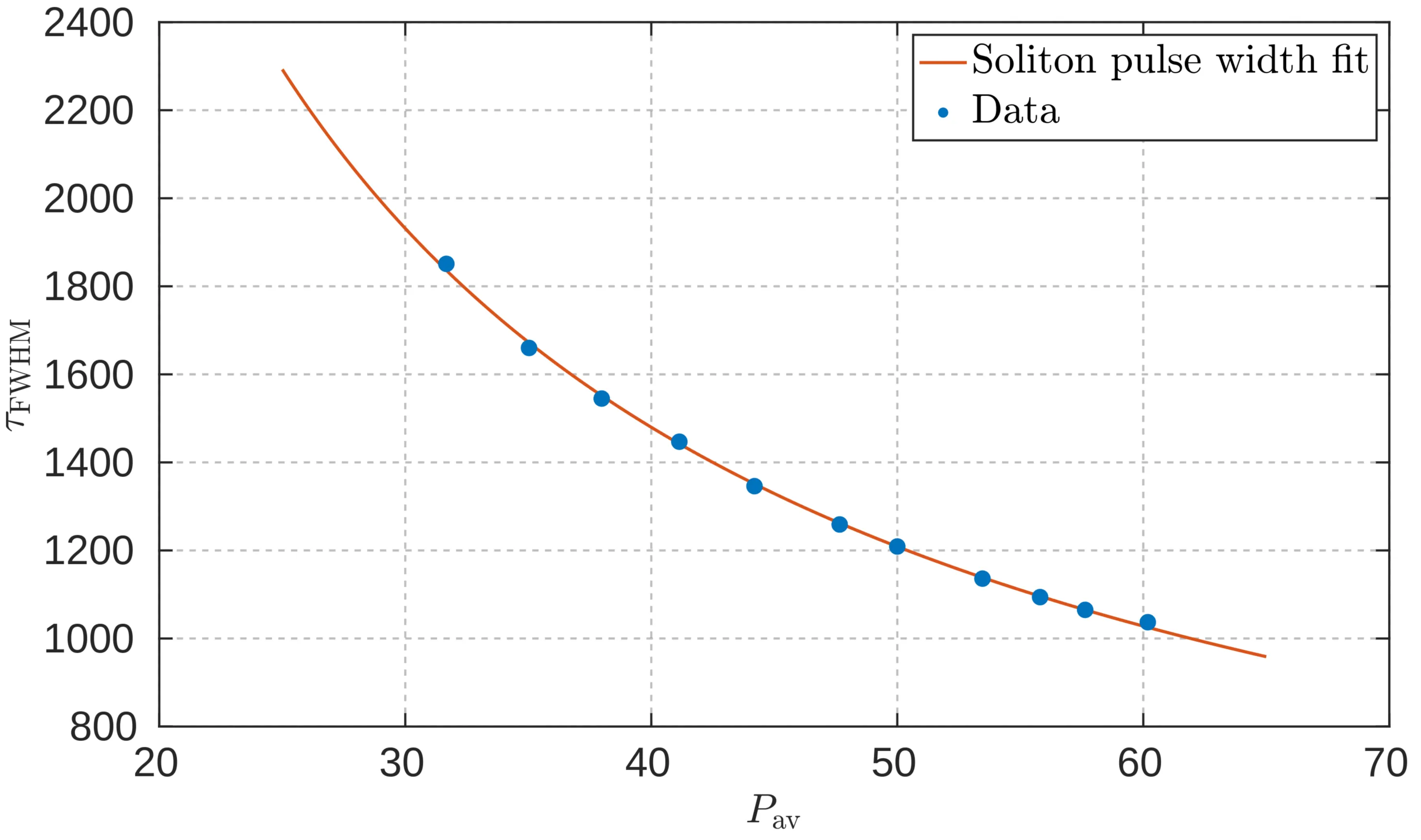
Measured pulse width as a function of average laser output power, fitted with an inverse power law $(1 / \bar{P})$ . The data represents the operating range of the laser between $33 W$ and $60 W$ , where stable modelocking occurs without CW breakthrough or other artefacts.

As the soliton FWHM pulse width follows the relationship

τ_{p} \sim \frac{1}{F_{p}} \sim \frac{1}{E_{p}} \sim \frac{1}{\bar{P}},

where $F_{p}$ is the pulse fluence and $E_{p}$ is the pulse energy, an inverse average power fit $(1 / P_{av})$ is applied across the range of $25 W$ to $60 W$ . This range corresponds to the operating conditions where the TDL is modelocked without continuous wave (CW) breakthrough or other artefacts.

Using this method, we can incorporate fluctuating peak powers and pulse widths into the simulation. Next, we compare the spectra with and without fluctuations. The next figure illustrates this comparison, showing that the ratio between these two spectra can be significant at specific wavelengths, resulting in substantial noise amplification, which we will refer to as noise gain moving forward.

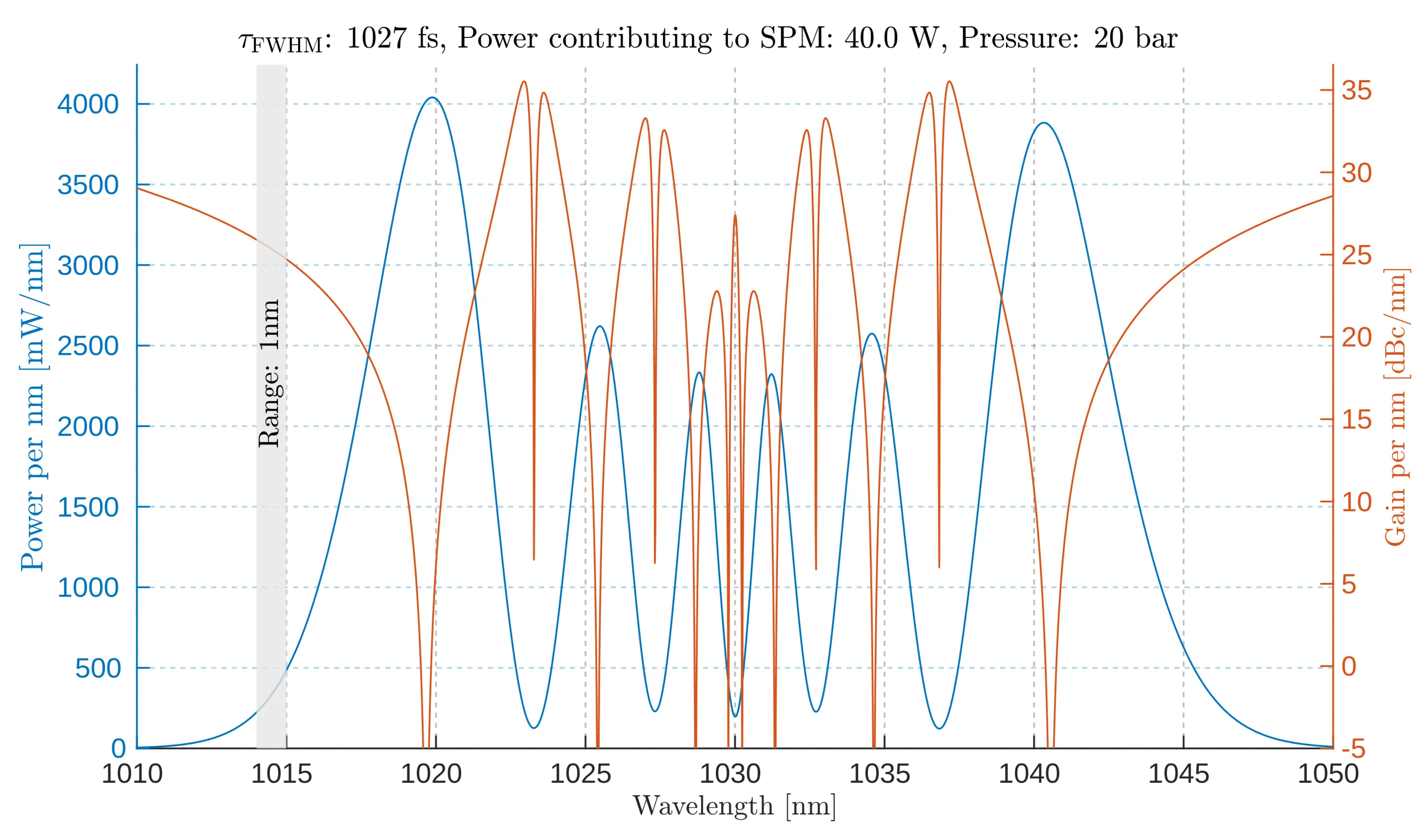
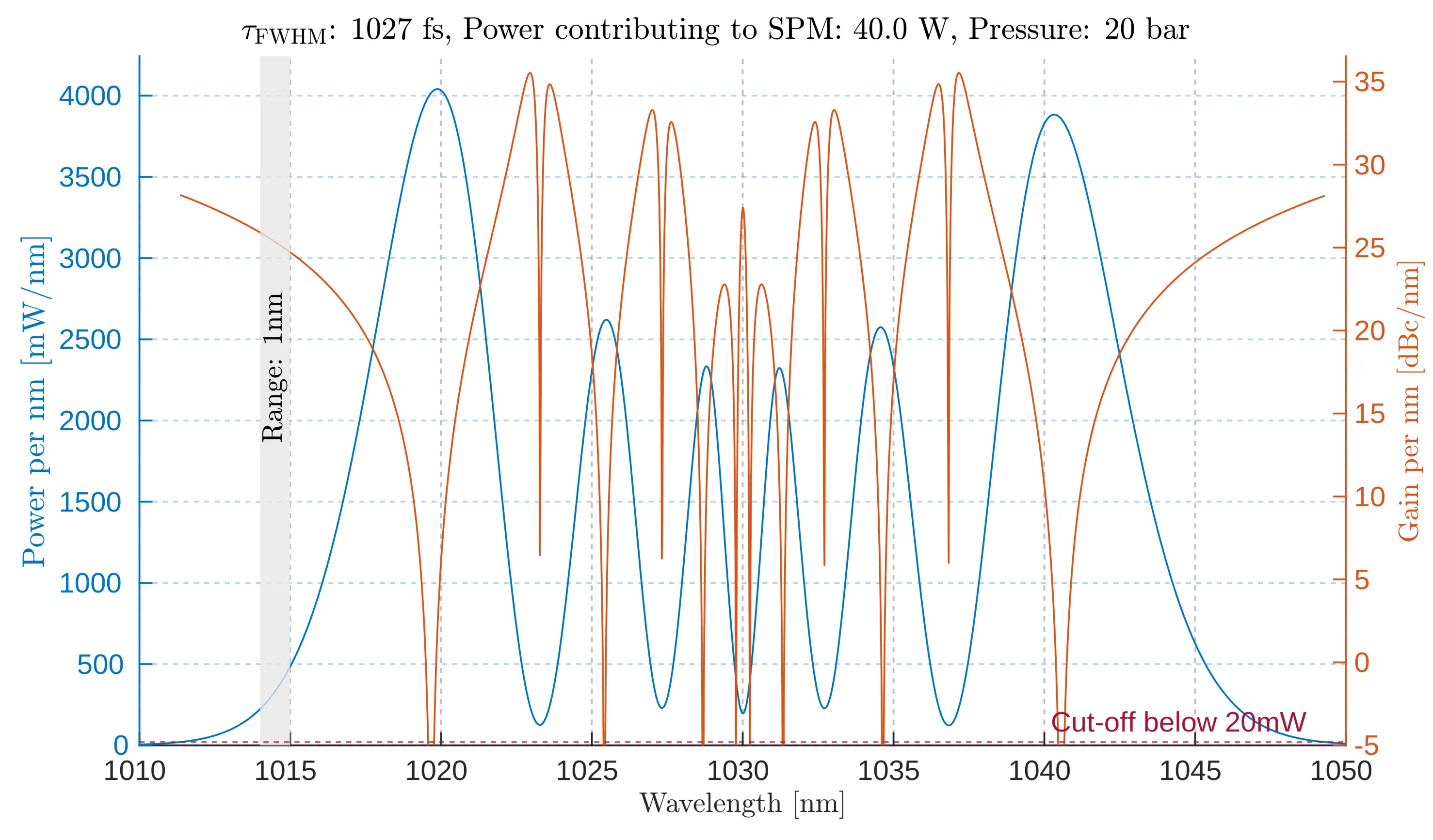
Attachments/Koeberlin_Master_Thesis 6.webp|700
Power density per nanometer (left, blue) and noise gain per nanometer (right, orange) as a function of wavelength. The power density reaches $4 W$ , while the noise gain peaks at $35 dB$ and maintains around $29 dB$ in the spectral wings. The fibre coupling efficiency is $82 %$ .

As the title indicates, "power contributing to SPM" refers to the power that efficiently couples into the fibre. The pulse width for simulation input is determined using the fitted relationship, based on the power coupled into the fibre, considering the presence of an output coupler for the diagnostics beam and an isolator.

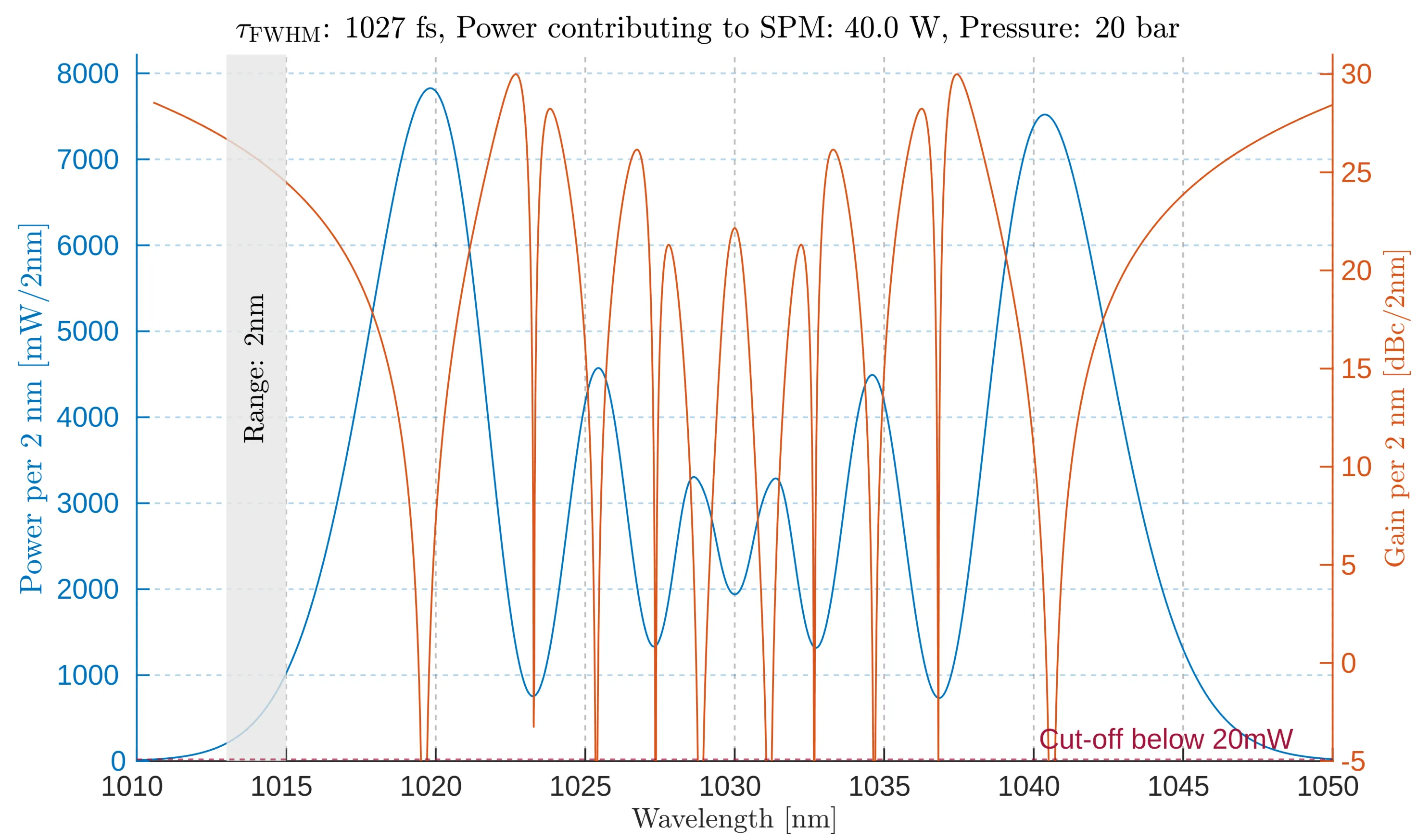
It is essential to note that the vertical axes represent gain and power per slice of one nanometer. This is significant because any measurement setup can only capture a finite spectral range. Increasing the slice interval to $2 nm$ will double the power within this range but will not necessarily result in a higher noise gain:

Attachments/Koeberlin_Master_Thesis 7.webp|700
Power density per two nanometers (left, blue) and noise gain per two nanometers (right, orange) as a function of wavelength. As expected, the power density reaches $8 W$ (doubling from the $1 nm$ slice), while the noise gain slightly decreases, peaking at $30 dB$ and $28 dB$ in the spectral wings. The fibre coupling efficiency is $82 %$ .

At larger intervals, spectral features become smeared, diminishing the distinct features of spectral broadening. Simulations indicate that a $1 nm$ spectral slice provides sufficient gain while remaining relatively simple to isolate.

We observe that at specific wavelengths, the relative change in intensity is significant (on the order of $35 dB$ ). We could potentially infer a lower shot noise level if we can measure the intensity change at these wavelengths. However, many high-gain points, especially on the spectrum's wings, correspond to low-intensity wavelengths, making them challenging to detect with the photodetectors used in this thesis. Even more critically, the reduced power at these outer wavelengths means that the power is counteracting the potential benefits of the high gain. To illustrate this effect, the following figure shows that most points in the wings disappear once we assume the detector requires a specific amount of power to measure a signal reliably:

Attachments/Koeberlin_Master_Thesis 8.webp|700
Power density per nanometer (left, blue) and noise gain per nanometer (right, orange) as a function of wavelength. The power density reaches $4 W$ , with the noise gain peaking at $35 dB$ . The imposed cut-off at $20 mW$ causes some points at the spectral wings to be inaccessible. The fibre coupling efficiency is $82 %$ .

Some high-gain points vanish due to low intensity, which numerical calculations and inherent rounding errors may artificially introduce. For the laser parameters (average power $\bar{P} = 60 W$ , FWHM pulse width $τ_{p} = 1027 fs$ , and pressure $p = 20 bar$ ), up to $29 dB$ of gain can still be achieved in the spectral wings. Interestingly, even when assuming a minimum required power per spectral slice and keeping all parameters constant except for the pressure, higher pressure does not necessarily result in a larger gain.

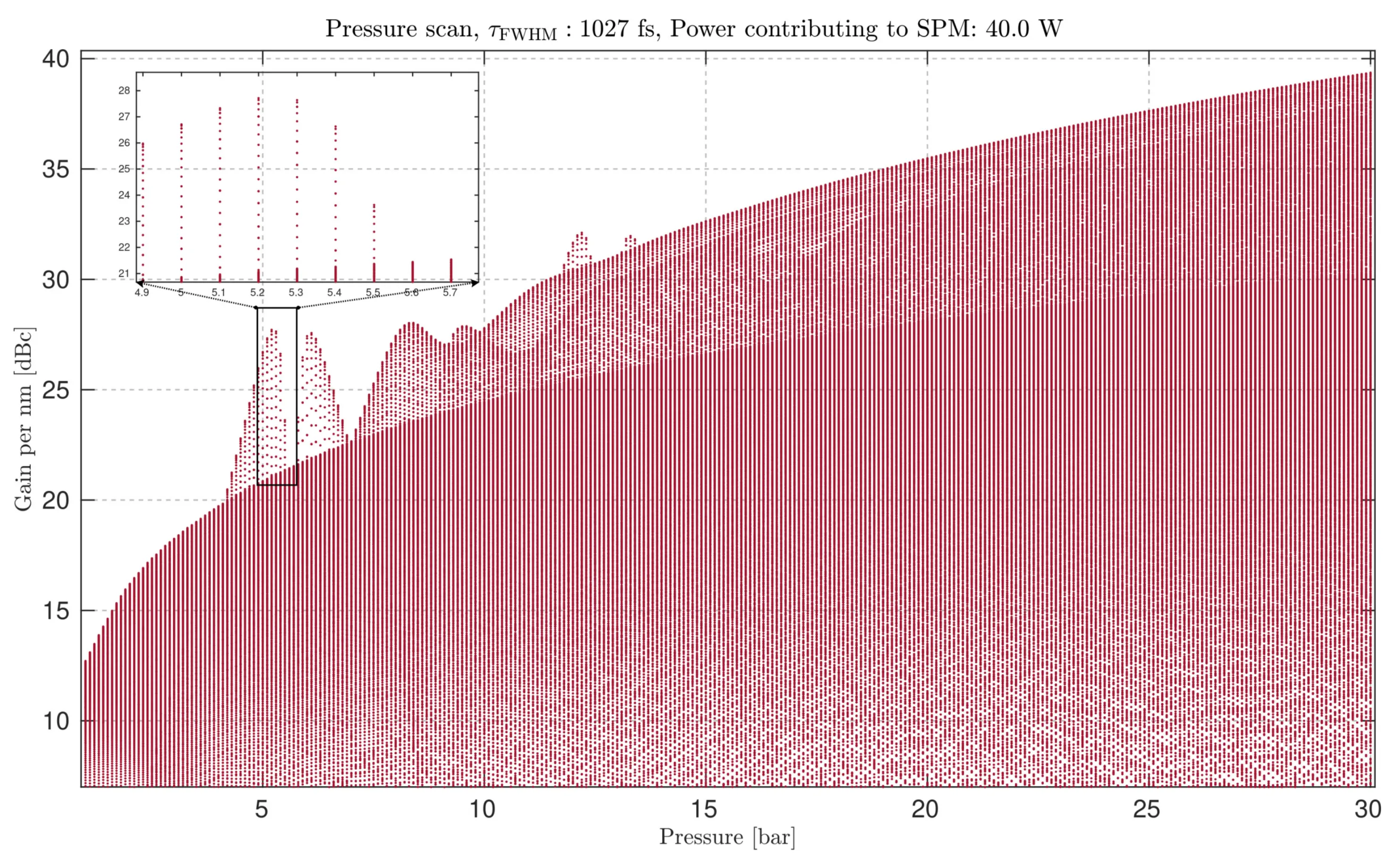
To illustrate this effect, the next figure presents a pressure scan ranging from $1$ to $30 bar$ in increments of $0.1 bar$ , with all other laser parameters held constant. The maximum achievable gain occurs at the highest pressure point, with a consistent increase from $15$ to $30 bar$ . However, note the gain density around $5.2 bar$ .

Attachments/Koeberlin_Master_Thesis 9.webp|700
Pressure scan from $1$ to $30 bar$ in steps of $0.1 bar$ . The simulation is run once for each pressure, and the gain density values are plotted along a vertical line. The parameters remain constant: $50 W$ input power, $82 %$ fibre coupling efficiency, and $1027 fs$ pulse width with a cut-off at $20 mW$ .

While this outlier may initially appear to be a numerical artefact, the next figure demonstrates that this point is located precisely at the centre of the broadened spectrum:

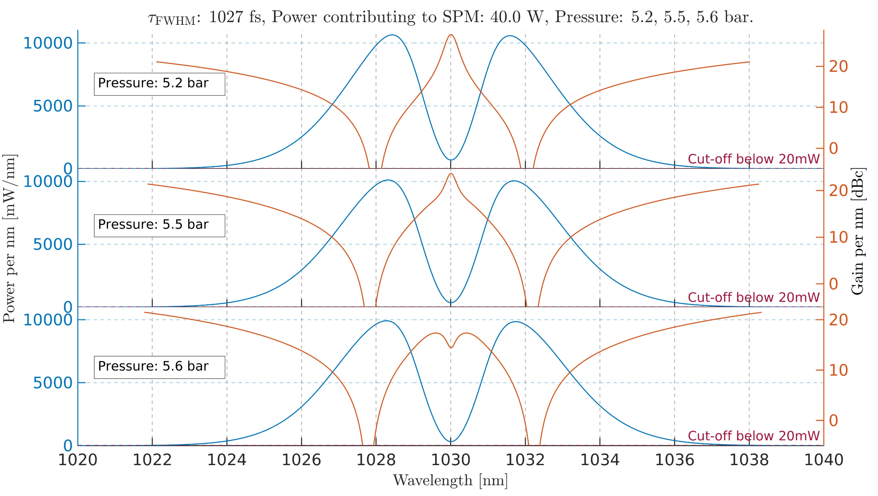
Attachments/Koeberlin_Master_Thesis 10.webp|700
Power density per nanometer (left, blue) and noise gain per nanometer (right, orange) as a function of wavelength for three different pressures: $5.2$ , $5.5$ , and $5.6 bar$ . The central peak starts to split around $5.6 bar$ , leading to a sudden change in maximum gain. The fibre coupling efficiency is $82 %$ .

Whenever the central peak "splits" into two new peaks, the maximum gain momentarily decreases before these new peaks become dominant, causing the pressure scan to follow a new trend. The noise gains for pressures of $5.2$ , $5.5$ , and $5.6 bar$ are stacked to show the significant change in maximum gain as the central peak begins to split.

2.7 Using Noise Gain from Spectral Broadening to Infer a Low Shot-Noise Level

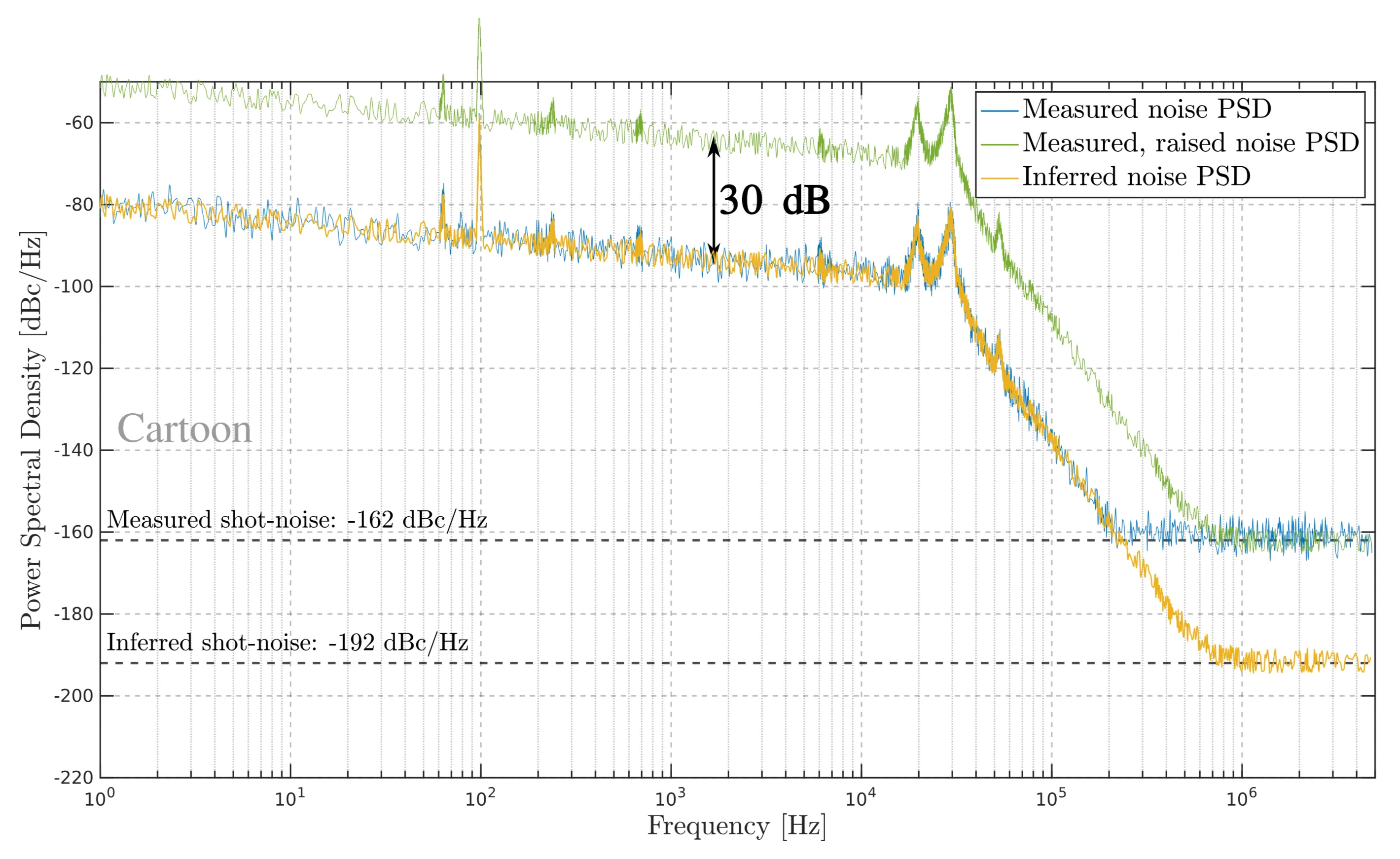
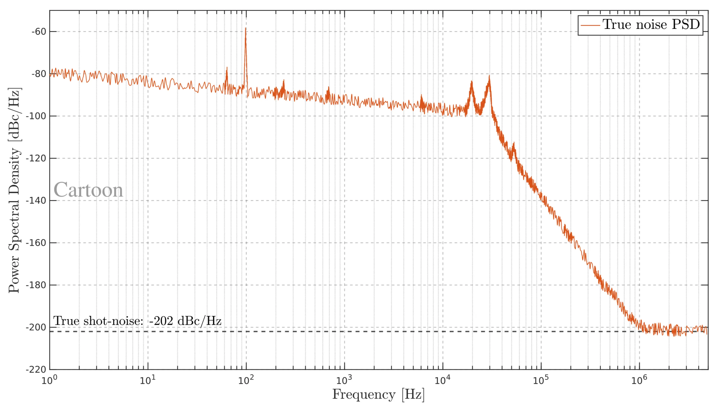
Now that the impact of spectral broadening on noise has been discussed, it is crucial to explain how this technique can be used to infer a low shot-noise level. To illustrate this, the next six figures demonstrate the step-by-step process for estimating a low shot-noise level. The noise trace used in these figures is generated for illustrative purposes.

This procedure requires only a single photodiode, a method to raise the noise PSD uniformly across all frequencies, and two measurements: one of the laser before spectral broadening and one after. The strength of this method is that the measurement challenge is shifted from the detection setup to obtaining the uniform noise gain.

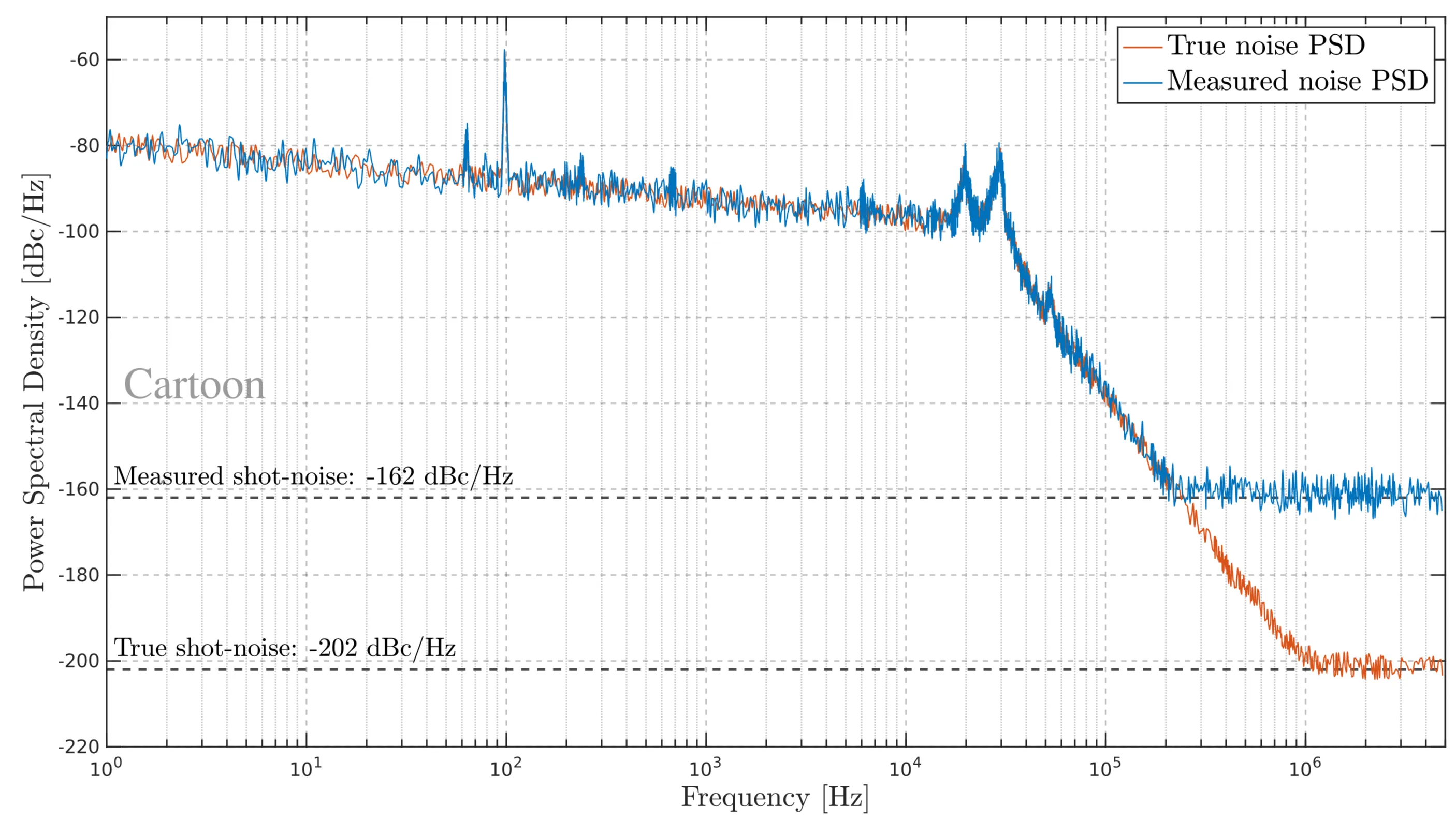
Step 1: Assumed noise PSD of a $60 W$ laser, running into the shotnoise limit of $- 202 dBc / Hz$ around $1 MHz$ . To obtain this noise trace, one must measure the full $60 W$ of optical power with a photodiode, which is impractical.
Attachments/Koeberlin_Master_Thesis 11.webp|700

Step 2: Assuming the photodiode can only measure up to $10 mW$ of optical power, the shot-noise limit would be at $- 162 dBc / Hz$ . In the laboratory, the blue noise PSD would be measured, following the true noise PSD but hitting the detector-limited shot-noise threshold earlier.
Attachments/Koeberlin_Master_Thesis 12.webp|700

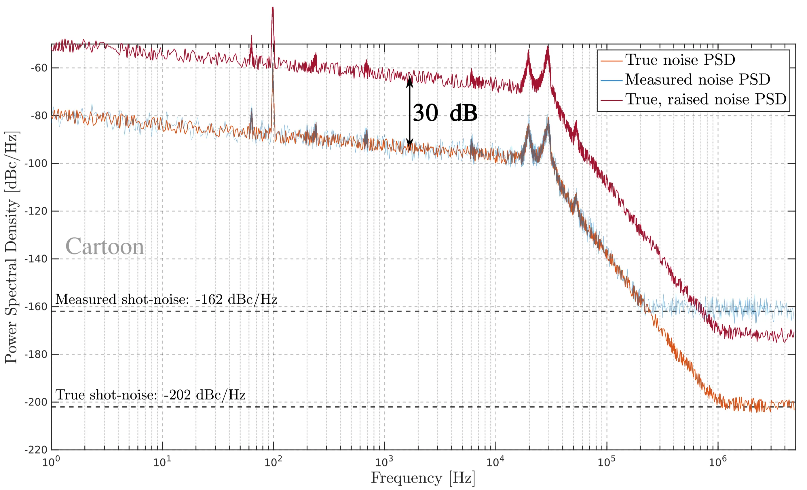
Step 3: Now assume a tool (in this case, spectral broadening) exists that uniformly raises the entire noise PSD by a fixed amount - in this case, $30 dB$ . As a result, the true noise PSD (orange) would shift upwards by $30 dB$ across all frequencies (red).
Attachments/Koeberlin_Master_Thesis 13.webp|700

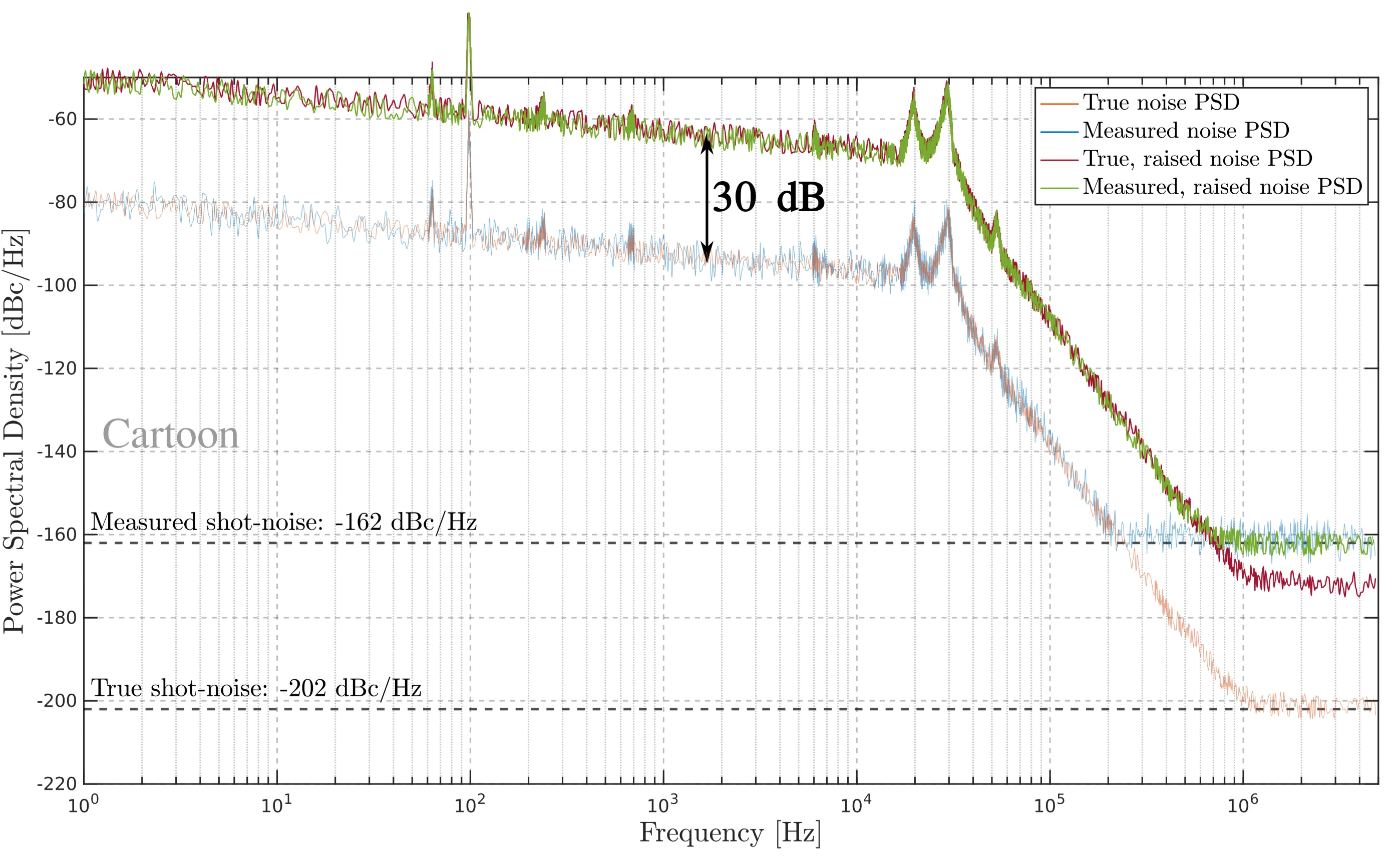
Step 4: Repeating the noise measurement with the laser that has its noise increased, the green curve is obtained in the lab. The measured noise trace will still be limited by the photodiode's shot-noise threshold at $- 162 dBc / Hz$ , but this occurs at a higher frequency due to the increased noise.
Attachments/Koeberlin_Master_Thesis 14.webp|700

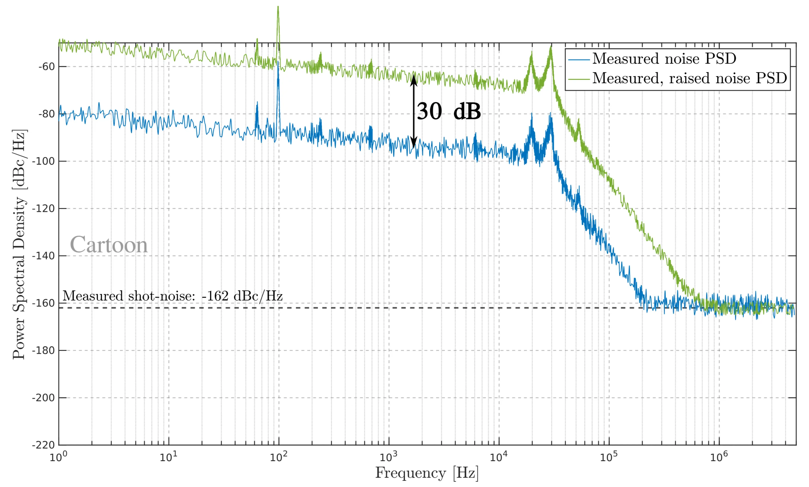
Step 5: After conducting measurements on both the original laser and the noisy laser, the blue and green curves are. They are consistently spaced apart by $30 dB$ . A low shot-noise limit can be inferred based on the assumption that the noise gain equally affects all frequencies (see step 6).
Attachments/Koeberlin_Master_Thesis 15.webp|700

Step 6: Given the assumption that the noise gain increases the noise PSD by $30 dB$ uniformly across all frequencies, we infer that the true shotnoise limit is at $- 192 dBc / Hz$ .
Attachments/Koeberlin_Master_Thesis 16.webp|700