Jump back to chapter selection.

Table of Contents

3.1 Characterisation of Ultrashort Pulses
3.2 RABBITT: Reconstruction of Attosecond Beating by Interference of Two-Photon Transitions
3.3 Attosecond Pulse Characterisation: FROG-CRAB
3.4 Control of Amplitude and Phase of an APT
3.5 Temporal Information Extracted from Attosecond Pulse Train (APT) Photoionisation Experiments
3.6 PROBE and PROBD
3.7 From RABBITT to Streaking Regime

3 Characterisation and Control of Attosecond Pulses

Before diving into the specifics of characterising attosecond pulses, it is instructive to briefly review the characterisation of more conventional ultrashort (femtosecond) optical pulses, as many underlying principles and challenges are related.

3.1 Characterisation of Ultrashort Pulses

3.1.1 Autocorrelation

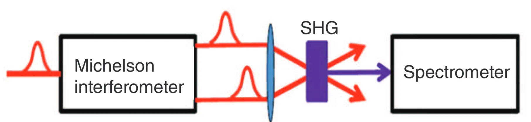
The duration of short optical pulses can be readily estimated using the technique of autocorrelation. In a common setup, a pulse is split into two identical replicas, and these replicas are then made to overlap spatially inside a nonlinear crystal (often one that allows second-harmonic generation, SHG), with a variable relative time delay $\tau$ between them. The intensity of the second-harmonic signal generated is proportional to the product of the intensities of the two overlapping pulse replicas. The measured SHG signal as a function of delay is the intensity autocorrelation:

This signal is non-zero only when the two pulse replicas overlap in time within the crystal. The width of the autocorrelation trace provides an estimate of the pulse duration (after deconvolution with a factor that depends on the pulse shape). However, it is important to note that this method only yields an estimate of the pulse duration and contains no information about the actual temporal profile of the pulse or its phase. Complete pulse characterisation requires knowledge of the spectral phase $\mathrm{\Phi }(\omega )$ in addition to the spectral amplitude $|\tilde{E}(\omega )|$, such that the complex spectral field is $\tilde{E}(\omega )=|\tilde{E}(\omega )|e^{i\mathrm{\Phi }(\omega )}$. The temporal electric field $E(t)$ can then be obtained via an inverse Fourier transform. The spectral amplitude $|\tilde{E}(\omega )|$ (or rather, the spectral intensity $|\tilde{E}(\omega ){|}^2$) can be measured with a spectrometer. The principal challenge is then to measure the spectral phase $\mathrm{\Phi }(\omega )$. The next two methods, FROG and SPIDER, are designed for this purpose and are also discussed in my Ultrafast Laser Physics notes, albeit in greater detail and from a slightly different perspective.

3.1.2 FROG: Frequency-Resolved Optical Gating

The most widely used implementation of Frequency-Resolved Optical Gating (FROG) is SHG-FROG. In this technique, similar to autocorrelation, two replicas of the pulse $E(t)$ with a relative delay $\tau$ are focused into an SHG crystal. However, instead of just measuring the total SHG energy, the spectrum of the SHG signal $E_{SHG}(t,\tau )\sim E(t)E(t-\tau )$ is measured for each delay $\tau$. The resulting FROG trace is a two-dimensional plot of this spectrally resolved SHG signal:

Here, ${\omega }_{\text{SHG}}$ is the frequency variable in the SHG spectrum, and the Fourier transform kernel $e^{-i{\omega }_{\text{SHG}}t}$ is used by convention for spectral analysis. This method can be considered a type of amplitude gating, where one pulse effectively gates the other within the SHG crystal, and the conversion efficiency depends nonlinearly on the laser intensity. The schematic setup of SHG-FROG often involves a Michelson interferometer to introduce the delay $\tau$.

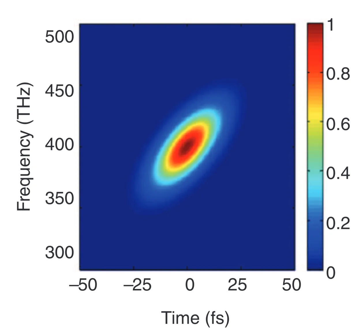
The FROG trace is a spectrogram of the pulse, containing information about both its amplitude and phase.

To retrieve the pulse's electric field $E(t)$ (both amplitude and phase) from the measured FROG trace, an iterative phase-retrieval algorithm is employed. The FROG trace provides a highly redundant dataset, sampling the pulse in both time (via $\tau$) and frequency (via ${\omega }_{\text{SHG}}$). While this redundancy makes the retrieval robust against noise and less prone to ambiguities, the method can be sensitive to detector uniformity and calibration, and the iterative algorithm requires computational effort.

3.1.3 SPIDER: Spectral Phase Interferometry for Direct Electric-Field Reconstruction

Another powerful method for complete pulse characterisation is SPIDER. It is based on spectral interferometry, measuring the interference pattern in the frequency domain between a pulse and a replica of itself that has been shifted both in time (by $\tau$) and in frequency (by a spectral shear $\mathrm{\Omega }$). The measured spectral interferogram $I(\omega )$ is:

From this interferogram, the phase term $\phi (\omega )=\mathrm{\Phi }(\omega )-\mathrm{\Phi }(\omega -\mathrm{\Omega })-\omega \tau$ can be extracted directly using Fourier-transform spectral interferometry techniques (filtering out the AC component in the "pseudo-time" domain obtained by Fourier transforming $I(\omega )$). The known delay $\tau$ and shear $\mathrm{\Omega }$ allow for the reconstruction of the spectral phase $\mathrm{\Phi }(\omega )$ by concatenation or integration of the phase differences $\mathrm{\Phi }(\omega )-\mathrm{\Phi }(\omega -\mathrm{\Omega })$.
To generate the required spectral shear $\mathrm{\Omega }$ between two time-delayed replicas of the pulse to be measured, these replicas are typically mixed with a strongly chirped auxiliary pulse in a nonlinear optical crystal (sum-frequency generation or difference-frequency generation). Each replica mixes with a different quasi-monochromatic slice of the chirped pulse, resulting in upconverted (or downconverted) pulses that are spectrally shifted relative to each other by $\mathrm{\Omega }$.

SPIDER is a non-iterative and relatively fast method, directly yielding the spectral phase.

3.2 RABBITT: Reconstruction of Attosecond Beating by Interference of Two-Photon Transitions

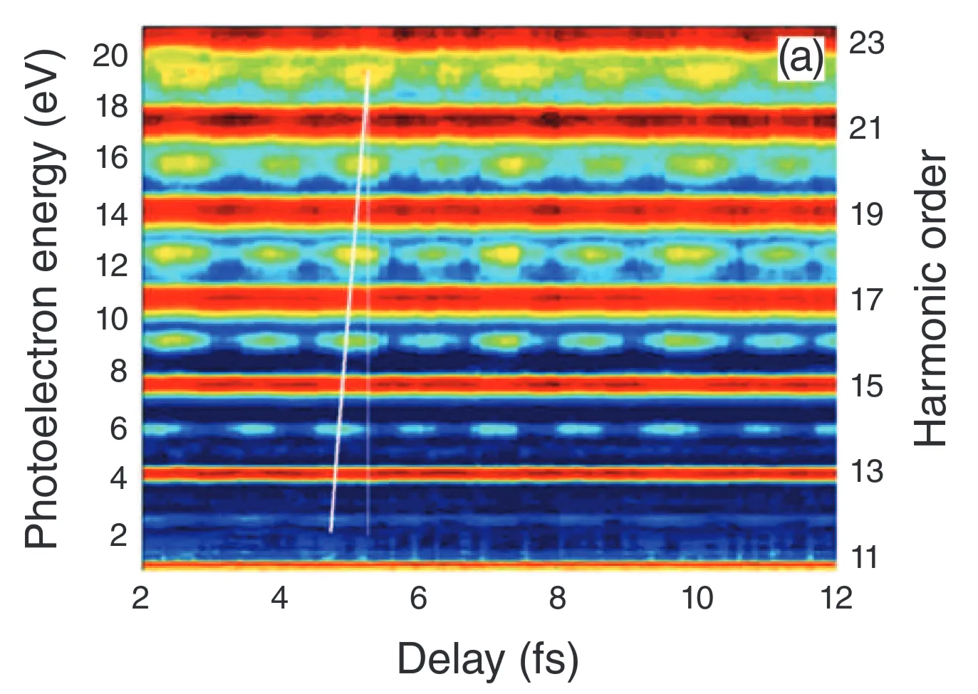
The RABBITT technique enables the determination of the relative spectral phases of the harmonics within an attosecond pulse train (APT). It involves probing the photoionisation of a target gas by the APT in the presence of a time-delayed, weak portion of the fundamental infrared (IR) laser field that was used to generate the harmonics. The intensity of the XUV harmonics is typically low enough that ionisation occurs primarily through single-photon absorption (a linear process in XUV intensity).

In the absence of the IR field, the photoelectron spectrum generated by the APT (consisting of odd harmonics $(2q+1){\omega }_0$) shows peaks at kinetic energies:

where ${\omega }_0$ is the fundamental laser frequency and $I_p$ is the ionisation potential of the target atom.
When the weak IR field (frequency ${\omega }_0$) is introduced, co-propagating with the XUV APT and with a controllable time delay $t_d$, the photoelectrons can additionally absorb or emit one IR photon during the ionisation process. This leads to the appearance of sidebands in the photoelectron spectrum, located at energies between the main harmonic peaks:

where $q^{\prime }$ is an integer. These sidebands correspond to two-photon transitions.

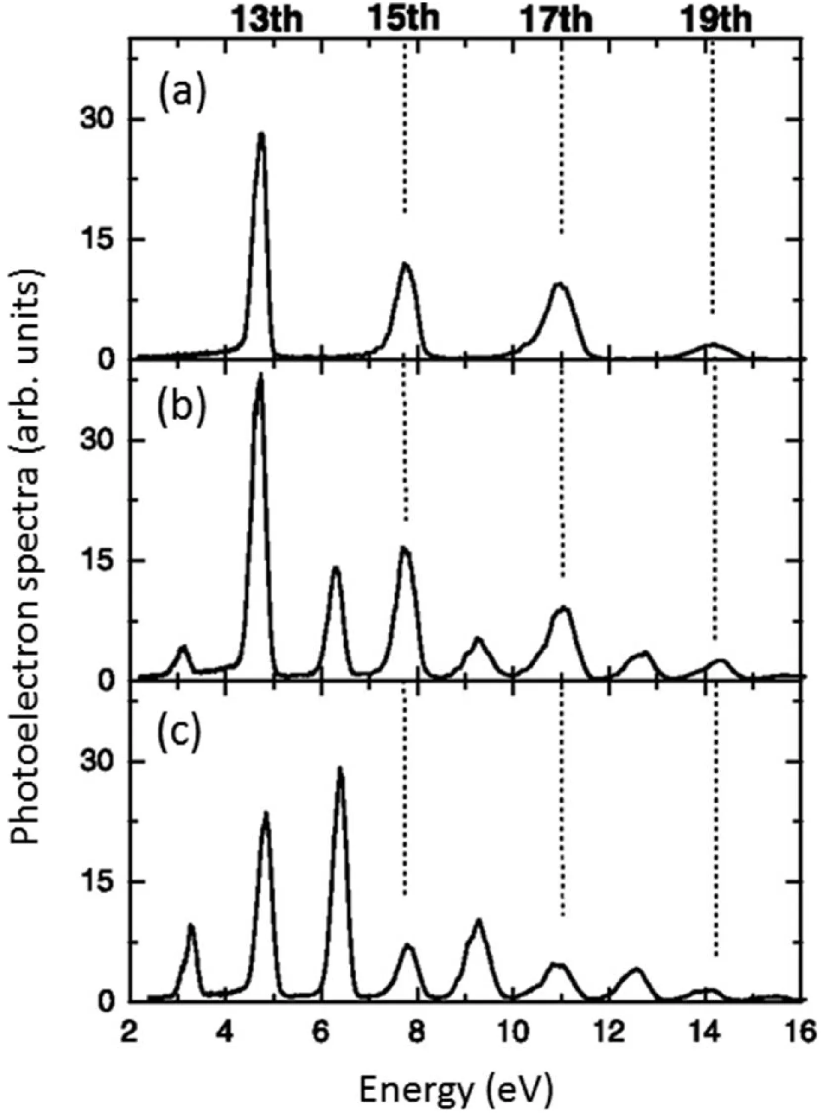
The figure shows photoelectron spectra of argon: (a) ionisation by XUV harmonics only; (b) and (c) with both XUV harmonics and the IR field, for two different XUV-IR delays. The amplitudes of the sidebands oscillate as a function of the delay $t_d$. This oscillation arises from the interference between two quantum paths leading to the same final photoelectron energy in a sideband $2q^{\prime }{\omega }_0$:

1. Absorption of a harmonic photon $(2q^{\prime }+1){\omega }_0$ followed by stimulated emission of an IR photon $(-{\omega }_0)$.
2. Absorption of a harmonic photon $(2q^{\prime }-1){\omega }_0$ followed by absorption of an IR photon $(+{\omega }_0)$.

The signal intensity $S_{2q^{\prime }}$ of a sideband (where $2q^{\prime }$ is the effective harmonic order of the sideband) can be expressed as:

Here:

• $A_{2q^{\prime }}$ and $B_{2q^{\prime }}$ are constants related to the transition amplitudes and harmonic intensities.
• ${\phi }_{2q^{\prime }+1}$ and ${\phi }_{2q^{\prime }-1}$ are the spectral phases of the two adjacent odd harmonics contributing to the sideband.
• $\mathrm{\Delta }{\phi }_{2q^{\prime }}^{\text{atomic}}$ is an additional phase contribution from the photoionisation process itself (the "atomic phase" or "continuum-continuum phase").

The sideband signal $S_{2q^{\prime }}(t_d)$ oscillates at twice the fundamental laser frequency ($2{\omega }_0$) as a function of $t_d$. By measuring this oscillation for each sideband, the phase difference between adjacent odd harmonics, $\mathrm{\Delta }{\phi }_{2q^{\prime }}^{\text{XUV}}={\phi }_{2q^{\prime }+1}-{\phi }_{2q^{\prime }-1}$, can be extracted (assuming $\mathrm{\Delta }{\phi }_{2q^{\prime }}^{\text{atomic}}$ is known or can be reasonably estimated/neglected for relative XUV phase retrieval). This allows the reconstruction of the group delay dispersion of the APT.
The term ${\tau }_{\text{RABBITT}}$ sometimes refers to the phase offset of the $2{\omega }_0$ oscillation, which includes both the XUV phase difference and the atomic phase. Interpreting this delay requires careful consideration of the quantum pathways. It has been shown that this delay can be related to the photoemission time delay.

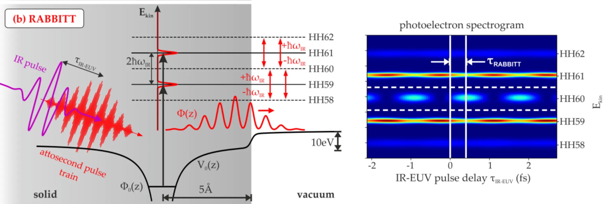
The RABBITT method is sensitive to any chirp present in the XUV pulse train (variation of harmonic phases) and also to the chirp of the IR probe pulse, making it a powerful diagnostic.

3.3 Attosecond Pulse Characterisation: FROG-CRAB

While RABBITT is suited for characterising attosecond pulse trains, different techniques are needed for single attosecond pulses (SAPs), especially those with continuous spectra. A prominent method is FROG-CRAB (Frequency-Resolved Optical Gating for Complete Reconstruction of Attosecond Bursts).
The goal is to determine the full electric field of the SAP, $E_{\text{XUV}}(t)$, or equivalently its complex spectrum ${\tilde{E}}_{\text{XUV}}(\omega )=U(\omega )e^{i\mathrm{\Phi }(\omega )}$, where $U(\omega )$ is the spectral amplitude and $\mathrm{\Phi }(\omega )$ is the spectral phase. The temporal intensity profile is $I(t)=|E_{\text{XUV}}(t){|}^2$, and the temporal phase (which may include an attochirp) is $\varphi (t)=\arg [E_{\text{XUV,analytic}}(t)]-{\omega }_{X}t$, where ${\omega }_X$ is the central XUV frequency.

Traditional femtosecond characterisation methods (autocorrelation, SPIDER, FROG) are generally not directly applicable to attosecond XUV pulses due to the lack of suitable fast detectors or efficient nonlinear optical materials in the XUV range, and the typically low photon flux of SAPs. Attosecond pulse characterisation therefore often relies on cross-correlation techniques where the SAP interacts with a time-delayed, intense, few-cycle infrared (IR) field (often the same laser used for HHG). The XUV pulse ionises a target gas, creating photoelectrons. The co-propagating, time-delayed IR field then "streaks" these photoelectrons, meaning it modifies their final momentum (and thus kinetic energy) depending on the instantaneous vector potential of the IR field at the moment of ionisation and during the electron's departure.

3.3.1 Attosecond Streaking and the Strong-Field Approximation

The core of FROG-CRAB is attosecond streaking. A single attosecond XUV pulse ionises atoms from a target gas. A synchronised, intense few-cycle IR laser pulse, with a variable time delay $\tau$ relative to the XUV pulse, interacts with the photoelectron wavepacket created by the XUV pulse. This IR "streaking" field changes the final momentum of the emitted electrons. By measuring the photoelectron kinetic energy spectrum as a function of the delay $\tau$, a 2D plot called a streaking spectrogram (or trace) is generated. This spectrogram contains encoded information about the temporal profile of the XUV pulse and the electric field of the IR streaking pulse.

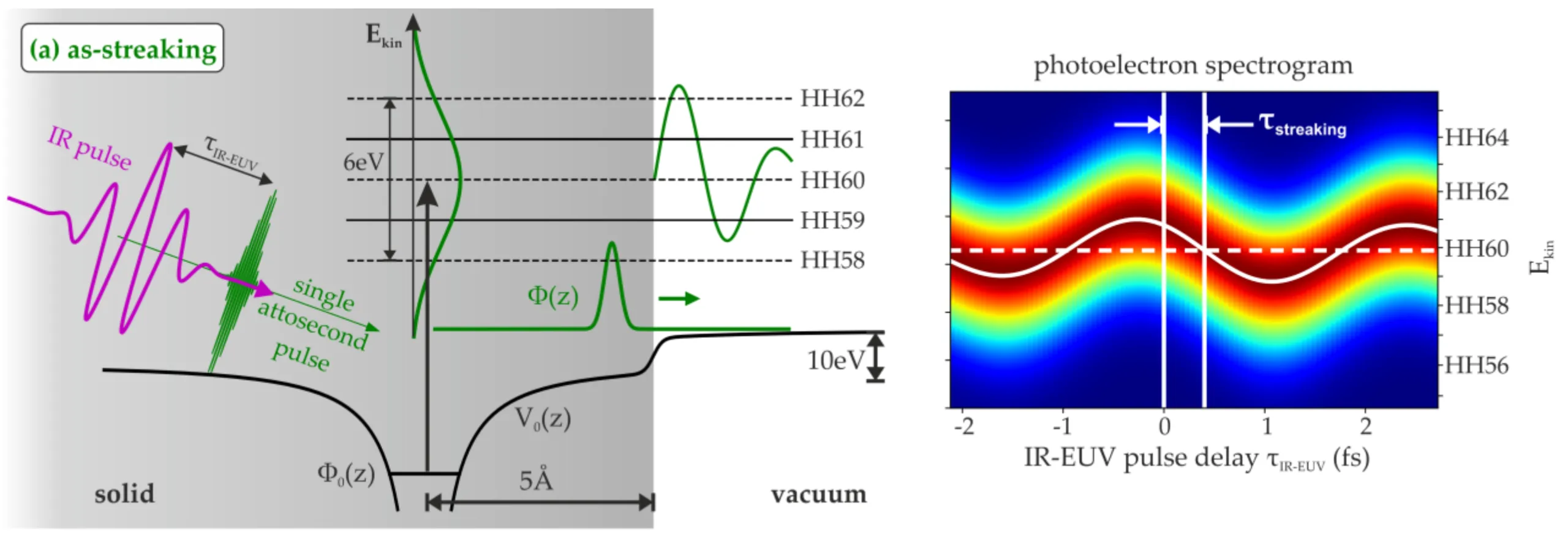
Key differences from RABBITT include:

• The IR field in streaking is typically much stronger than in RABBITT, allowing it to significantly alter electron momenta rather than just enabling weak sideband transitions.
• Streaking is primarily used for SAPs with continuous (or quasi-continuous) spectra, whereas RABBITT analyses discrete harmonics in an APT.
• While both involve a photoemission delay, the interpretation in streaking can often be approached with a more classical picture for the electron's motion in the IR field after ionisation, whereas RABBITT explicitly relies on quantum interference.

A quantum mechanical description of attosecond streaking typically employs the Strong-Field Approximation (SFA). The SFA involves several key assumptions:

1. Single Active Electron Approximation: Only one electron participates in the ionisation.
2. Neglect of Coulomb Potential in Continuum: Once ionised, the photoelectron's motion is governed solely by the laser fields; the influence of the parent ion's Coulomb potential is neglected.
3. Two-Step Model: Transition is from the ground state directly to Volkov continuum states (dressed by the IR field); influence of other bound atomic states is ignored.

Within the SFA, the transition amplitude $a_{\mathbf{v}}(\tau )$ for a photoelectron to reach a final momentum $\mathbf{v}$ (and kinetic energy $W={\mathbf{v}}^2/2$ in atomic units) can be expressed as:

where $S(t)=(W+I_p)t-{\int }_t^{\mathrm{\infty }}d{t}^{\prime }[\mathbf{v}\cdot {\mathbf{A}}_{\text{IR}}(t^{\prime })+{\mathbf{A}}_{\text{IR}}^2(t^{\prime })/2]$.
Here:

• $\tau$ is the XUV-IR delay.
• ${\mathbf{E}}_X(t-\tau )$ is the electric field of the XUV pulse.
• ${\mathbf{A}}_{\text{IR}}(t)$ is the vector potential of the IR field.
• $\mathbf{p}(t)=\mathbf{v}+{\mathbf{A}}_{\text{IR}}(t)$ is the instantaneous kinetic momentum.
• ${\mathbf{d}}_{\mathbf{p}(t)}$ is the dipole transition matrix element to the continuum state with momentum $\mathbf{p}(t)$.
• $I_p$ is the ionisation potential.
  The term $-{\int }_t^{\mathrm{\infty }}d{t}^{\prime }[\mathbf{v}\cdot {\mathbf{A}}_{\text{IR}}(t^{\prime })+{\mathbf{A}}_{\text{IR}}^2(t^{\prime })/2]$ is the Volkov phase, representing the phase accumulated by the electron in the IR field after ionisation. The IR field's primary role is to induce this ultrafast phase modulation on the electron wavepacket launched by the XUV pulse.

FROG-CRAB: A FROG Analogy

The measured photoelectron energy spectrum as a function of delay, $S(W,\tau )=|a_{\mathbf{v}}(\tau ){|}^2$, can be interpreted as a FROG-type trace. In FROG, a pulse $E(t)$ is gated by another pulse $G(t-\tau )$ to produce a signal field $E_{sig}(t,\tau )=E(t)G(t-\tau )$, whose spectrum is then measured: $S_{FROG}(\omega ,\tau )=|\int E_{sig}(t,\tau )e^{-i\omega t}dt{|}^2$.
By rearranging the SFA transition amplitude, it can be shown that the streaking spectrogram resembles a FROG trace where the XUV pulse effectively creates an initial electron wavepacket, and the IR field acts as a phase gate. This is the basis of FROG-CRAB.
To retrieve the temporal phase and intensity profile of the attosecond pulse, various iterative algorithms adapted from FROG, such as Principal Component Generalised Projection Algorithm (PCGPA), are used.

Central Momentum Approximation and Key Assumptions

A crucial simplification often made is the Central Momentum Approximation (CMA): the final momentum $\mathbf{v}$ in the Volkov phase is replaced by an average (or central) momentum ${\mathbf{v}}_0$. This makes the phase modulation ${\varphi }_{\text{IR}}(t)=-{\int }_t^{\mathrm{\infty }}d{t}^{\prime }[{\mathbf{v}}_0\cdot {\mathbf{A}}_{\text{IR}}(t^{\prime })+{\mathbf{A}}_{\text{IR}}^2(t^{\prime })/2]$ independent of the final electron energy for a given XUV pulse. Additionally, the dipole transition matrix element ${\mathbf{d}}_{\mathbf{p}(t)}$ is often assumed to be slowly varying with momentum over the bandwidth of the XUV pulse and constant in time during the XUV pulse. With these assumptions, the streaking spectrogram $S(W,\tau )$ can be processed using standard FROG algorithms.

The FROG-CRAB equation can then be written as:

where $E_{\text{XUV}}(t^{\prime }-\tau )$ is the XUV field launching an electron at $t^{\prime }$, $d_0$ is an effective (constant) dipole matrix element, and $e^{i{\varphi }_{\text{IR}}(t^{\prime })}$ is the phase gate from the IR field. The energy $W$ acts as the frequency variable. This allows simultaneous retrieval of $E_{\text{XUV}}(t)$ and the IR gating function (from which ${\mathbf{A}}_{\text{IR}}(t)$ can be derived).

FROG-CRAB offers significant advantages: versatility for different pulse types (isolated SAPs, APTs), robustness against noise due to information redundancy, and simultaneous characterisation of both XUV and IR pulses. The retrieved IR field can be cross-checked, validating the measurement.
However, limitations exist. Accurate reconstruction can be challenging for extremely short pulses (sub-100 as) or complex temporal structures (like satellite pulses), where SFA/CMA assumptions may falter. The technique is also sensitive to chirp on both XUV and IR pulses, which can manifest as distortions in the streaking trace.

3.4 Control of Amplitude and Phase of an APT

The RABBITT method determines the relative spectral phase $\mathrm{\Delta }{\phi }_{2q}^{\text{XUV}}={\phi }_{2q+1}-{\phi }_{2q-1}$ between adjacent harmonics in an APT. For perfectly transform-limited attosecond bursts within the train, all contributing harmonics should effectively be emitted simultaneously, meaning their group delay (attochirp) should be constant. The sideband oscillation in RABBITT can be written as:

where

is the XUV group delay difference centred around photon energy $2q{\omega }_0$. If this group delay $t_{2q}^e$ (often just called $t^e(\mathrm{\Omega })$ where $\mathrm{\Omega }=2q{\omega }_0$) is constant across all harmonics, they are effectively synchronised, resulting in TL pulses.

Experimental measurements often show that $t^e$ increases approximately linearly with photon energy for harmonics generated in the plateau region from the "short" quantum trajectory. This linear dependence indicates a positive chirp on the attosecond bursts, leading to temporal broadening. This intrinsic chirp primarily originates from the single-atom response. Macroscopic conditions, such as focusing the laser beam relative to the gas jet, can influence phase matching and preferentially select contributions from specific quantum trajectories (like short trajectories), which tend to have a more regular chirp.

Although experimental optimisation of HHG conditions can minimise this attochirp, it often cannot be completely eliminated at the source. To compensate for a positive chirp (where higher frequency components arrive later) accumulated during HHG, the generated APT can be propagated through a material or structure exhibiting negative group delay dispersion (GDD) in the XUV range. Thin metallic filters (such as aluminium, zirconium, or tin) can serve this purpose over specific XUV energy ranges, effectively compressing the attosecond bursts closer to their transform limit.

3.5 Temporal Information Extracted from Attosecond Pulse Train (APT) Photoionisation Experiments

In characterising APTs with the RABBITT method, the atomic phase contribution, $\mathrm{\Delta }{\phi }_{2q}^{\text{atomic}}$, to the sideband oscillation is typically calculated theoretically. For relative phase determination of the XUV harmonics, it is often assumed to be small or slowly varying and thus can sometimes be neglected or de-embedded. However, in studies aiming to probe photoionisation dynamics itself, extracting this atomic phase is the primary goal.
The photoionisation delay associated with the two-photon process contributing to the sideband $2q{\omega }_0$ can be defined as:

Using this, the sideband signal expression becomes:

The total measured phase shift of the $2{\omega }_0$ oscillation yields $t_{2q}^e+{\tau }_{2q}^{(2)}$. To isolate the intrinsic atomic delay ${\tau }_{2q}^{(2)}$, the XUV group delay $t_{2q}^e$ must be known or independently determined, for example by characterising the APT using photoionisation of a reference target with a well-known (or negligible) atomic delay. Alternatively, if the same XUV+IR pulse is used to ionise two different target species, or two distinct ionisation channels within the same target, the difference in their respective atomic delays, $\mathrm{\Delta }{\tau }^{(2)}$, can be found by comparing the $2{\omega }_0$ phase shifts from the two RABBITT measurements at the same photon energy.

The two-photon atomic delay, ${\tau }^{(2)}$, includes contributions from the interaction with the probing IR field (continuum-continuum transitions). For deeper insight into the field-free single-photon ionisation dynamics, it is desirable to isolate the phase information related purely to the single XUV photon absorption process. It can be shown that ${\tau }^{(2)}$ can often be approximated as:

where ${\tau }^{(1)}$ is the Wigner delay associated with the single-photon electronic wavepacket emission, and ${\tau }^{\text{cc}}$ is an IR-induced delay associated with continuum-to-continuum transitions. While ${\tau }^{\text{cc}}$ is generally target-independent, it can vary with photoelectron energy. This decomposition, though an approximation, can hold even when electron correlation effects are significant.

It is crucial to remember that the RABBITT method relies on the validity of second-order perturbation theory for the IR interaction, necessitating low IR intensities (typically $<{10}^{12}{\text{W/cm}}^2$) to avoid contributions from higher-order multi-photon processes to the sidebands. Moreover, the simplest interpretation of the derived equations is strictly valid when the ionised electron originates from an atomic s-state, where XUV absorption promotes the electron to an intermediate p-symmetry continuum wave. If the electron originates from a subshell with higher angular momentum (such as a p subshell), multiple intermediate continuum channels (for instance, s and d partial waves) can be accessed, leading to interference between different quantum paths for the two-photon transition. This interference results in more complex atomic delay dynamics that must be carefully considered.

3.6 PROBE and PROBD

While FROG-CRAB is a widely used and robust technique for characterising SAPs, it has two notable limitations:

1. The Central Momentum Approximation (CMA) can become inaccurate and restrict its applicability when characterising very broadband SAPs (where the XUV bandwidth is a significant fraction of its central energy).
2. The iterative retrieval algorithm used in FROG-CRAB might struggle to converge or yield accurate results, particularly when mid-IR pulses (with longer periods and more complex vector potentials over the XUV pulse duration) are employed as the streaking field.

In this section, two advanced retrieval methods, PROBD and PROOF, are introduced that aim to address these limitations. They can be more effective for broadband SAPs and can improve accuracy compared to standard FROG-CRAB under certain conditions.

3.6.1 PROBD

PROBD stands for Phase Retrieval Of Broadband Pulses by Deconvolution. The starting point is the same SFA-based equation for the streaking spectrogram $S(p,t_d)$ as used in the derivation of FROG-CRAB:

with the Volkov phase $\mathrm{\Phi }(p,t)$ defined as:

Unlike standard FROG-CRAB, PROBD aims to solve this equation without making the CMA (so without approximating $p$ by a constant $p_0$ in the Volkov phase $\mathrm{\Phi }(p,t)$). To make the iterative retrieval procedure more robust and accelerate convergence, the number of unknown parameters is minimised. These unknowns typically include the XUV pulse's spectral amplitude and phase, the IR field's vector potential (amplitude and phase), and potentially the atomic dipole transition matrix elements $d(p+A(t))$.

For broadband XUV pulse characterisation with PROBD, it is often assumed that the amplitude and phase of the dipole transition matrix elements $d(E^{\prime })$ can be accurately computed from atomic structure theory or are slowly varying and can be factored out. If the spectral amplitude of the XUV pulse $|E_{\text{XUV}}(\mathrm{\Omega })|$ can be independently determined (for instance, from XUV-only photoionisation measurements), then the primary remaining unknowns are the spectral phase of the XUV pulse and the vector potential (amplitude and phase) of the IR streaking field.

In PROBD, these unknown functions (XUV spectral phase and IR vector potential) are often expanded using a suitable basis set, such as B-spline functions:

where $g_i$ are the expansion coefficients to be retrieved, and $B_i^k(x)$ are the B-spline basis functions of order $k$. The iterative algorithm then searches for the coefficients $g_i$ that best reproduce the measured streaking spectrogram.

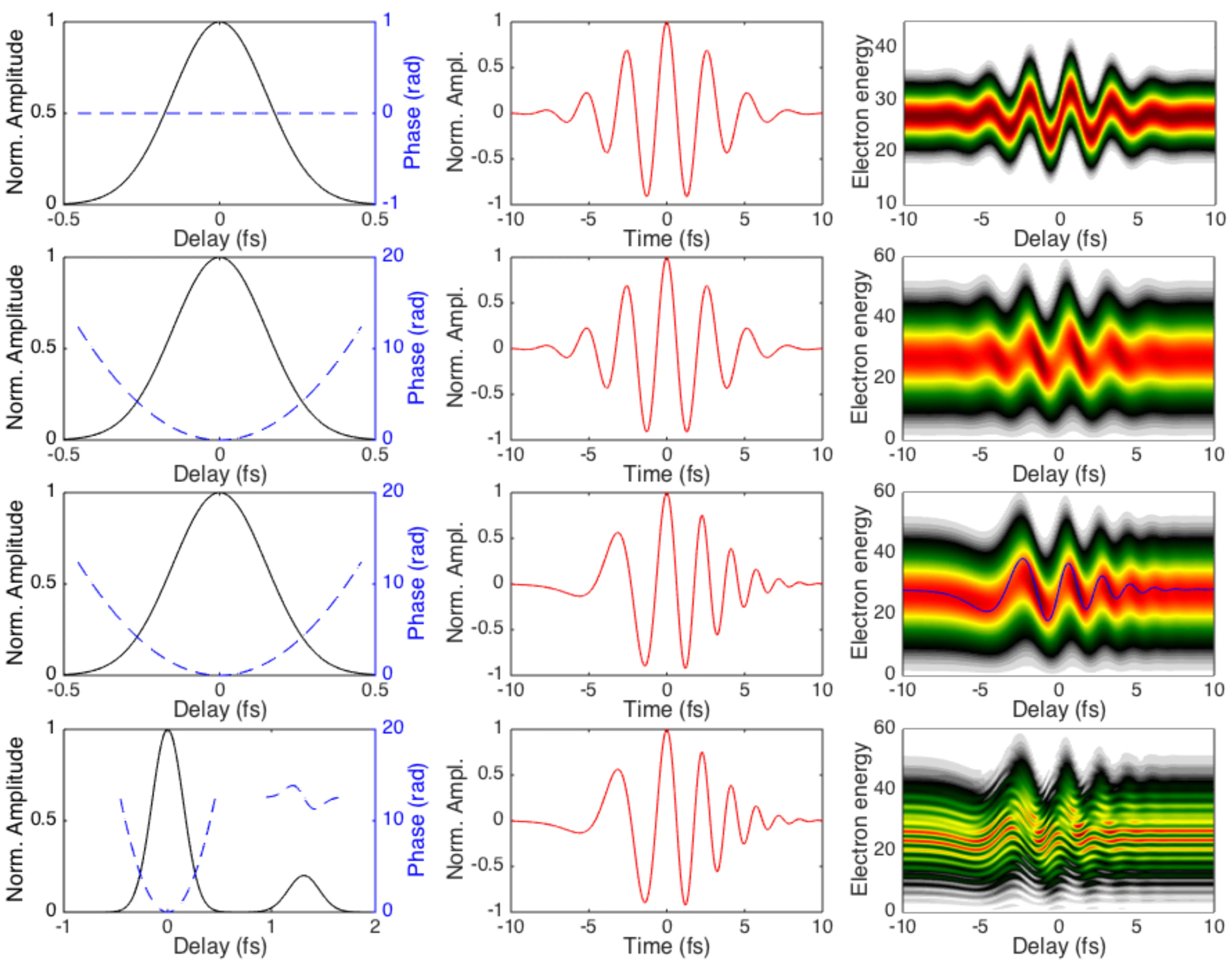
The following example illustrates an XUV pulse with a duration of 52 as, a central photon energy of 80 eV, and a spectral bandwidth of 90 eV. For such a broadband pulse, FROG-CRAB (relying on CMA) might fail to retrieve the XUV phase accurately, while PROBD, by avoiding CMA, could successfully reconstruct both the spectral phase and the time-domain intensity of the XUV pulse.

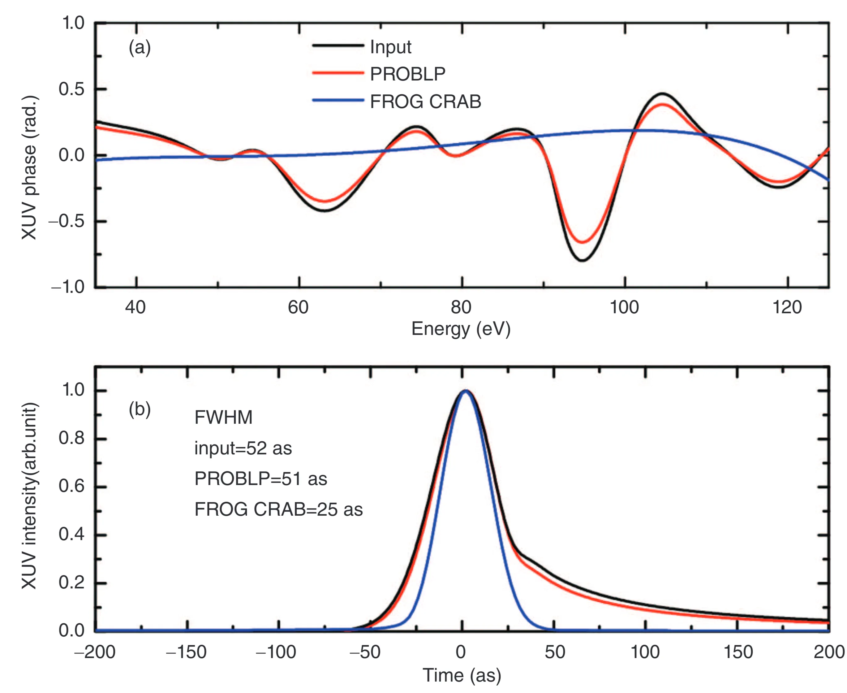
This example would clearly demonstrate that the CMA can be inadequate for very broadband XUV pulses.

3.6.2 PROOF

PROOF stands for Phase Retrieval by Omega Oscillation Filtering. It can be seen as a generalisation of the RABBITT technique applicable to the characterisation of single attosecond pulses (SAPs), particularly those with relatively continuous spectra. PROOF is most suitable when the IR streaking intensity is sufficiently weak to allow the use of second-order perturbation theory for modelling the interaction part of the streaking trace.

Consider photoelectrons detected along the polarisation axis of collinear XUV and IR pulses, and assume a monochromatic IR field for simplicity in the derivation. Under second-order perturbation theory, the streaking spectrogram $S(E,t_d)$ (where $E$ is final photoelectron kinetic energy) can be expressed as a sum of terms involving the XUV spectral field ${\tilde{E}}_{\text{XUV}}(\mathrm{\Omega })$ at different energies:

where higher-order terms in the IR field strength $E_{\text{IR,peak}}$ are neglected. Here:

• ${\mathrm{\Omega }}_0=E+I_p$ is the central XUV photon energy leading to photoelectron energy $E$ via one-photon absorption.
• ${\omega }_{\text{IR}}$ is the IR frequency.
• $d^{(1)}(E)$ is the transition dipole matrix element for single XUV photon absorption.
• $d^{(\pm )}(E)$ are the two-photon transition dipole matrix elements involving one XUV photon and the absorption ($+$) or emission ($-$) of one IR photon.

Expanding this expression to the lowest orders in $E_{\text{IR,peak}}$ that involve interference, we obtain:

where $S_{\text{XUV}}(E)=|{\tilde{E}}_{\text{XUV}}({\mathrm{\Omega }}_0)d^{(1)}(E){|}^2$ represents the XUV-only photoionisation signal, and $S_{\text{FSI}}(E,t_d)$ is the "first-second order interference" term, which contains the oscillations due to the IR field:

For a fixed electron energy $E$, the FSI term $S_{\text{FSI}}(E,t_d)$ oscillates with the delay $t_d$ primarily at the IR frequency ${\omega }_{\text{IR}}$ (and potentially $2{\omega }_{\text{IR}}$ if higher order terms in $E_{IR}$ were kept from the squared modulus). This oscillatory part can be written as:

where the amplitudes $A(E),B(E)$ and phases ${\mathrm{\Psi }}_{\text{abs/em}}(E)$ depend on the XUV spectral amplitude and phase differences, and the dipole matrix elements.
From the experimental spectrogram $S(E,t_d)$, the FSI term can be isolated by Fourier filtering the data (for each $E$) with respect to $t_d$ to extract the component oscillating at ${\omega }_{\text{IR}}$. This approach forms the basis of the PROOF method for retrieving XUV pulse characteristics.

Since PROOF operates in the weak IR field regime (intensities typically below ${10}^{12}{\text{W/cm}}^2$), the streaking effect (energy shift) is relatively small. This can lead to a lower signal-to-noise ratio for the oscillatory component, which may introduce uncertainties in the retrieved phase of the SAP. Nevertheless, PROOF provides an effective method for phase retrieval in weak-field conditions where SFA might be less accurate or when simpler analysis is desired, expanding the toolkit of attosecond metrology.

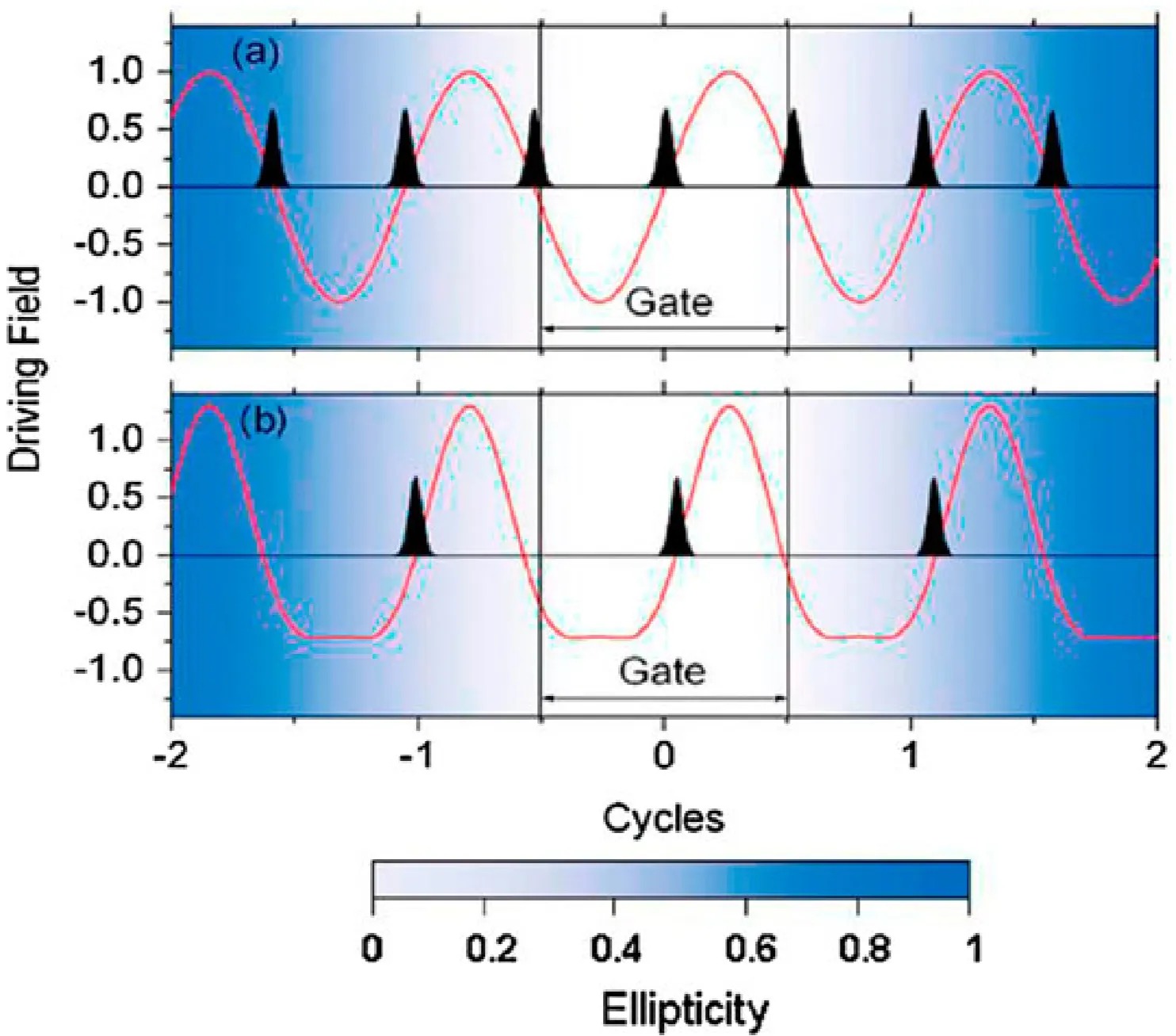
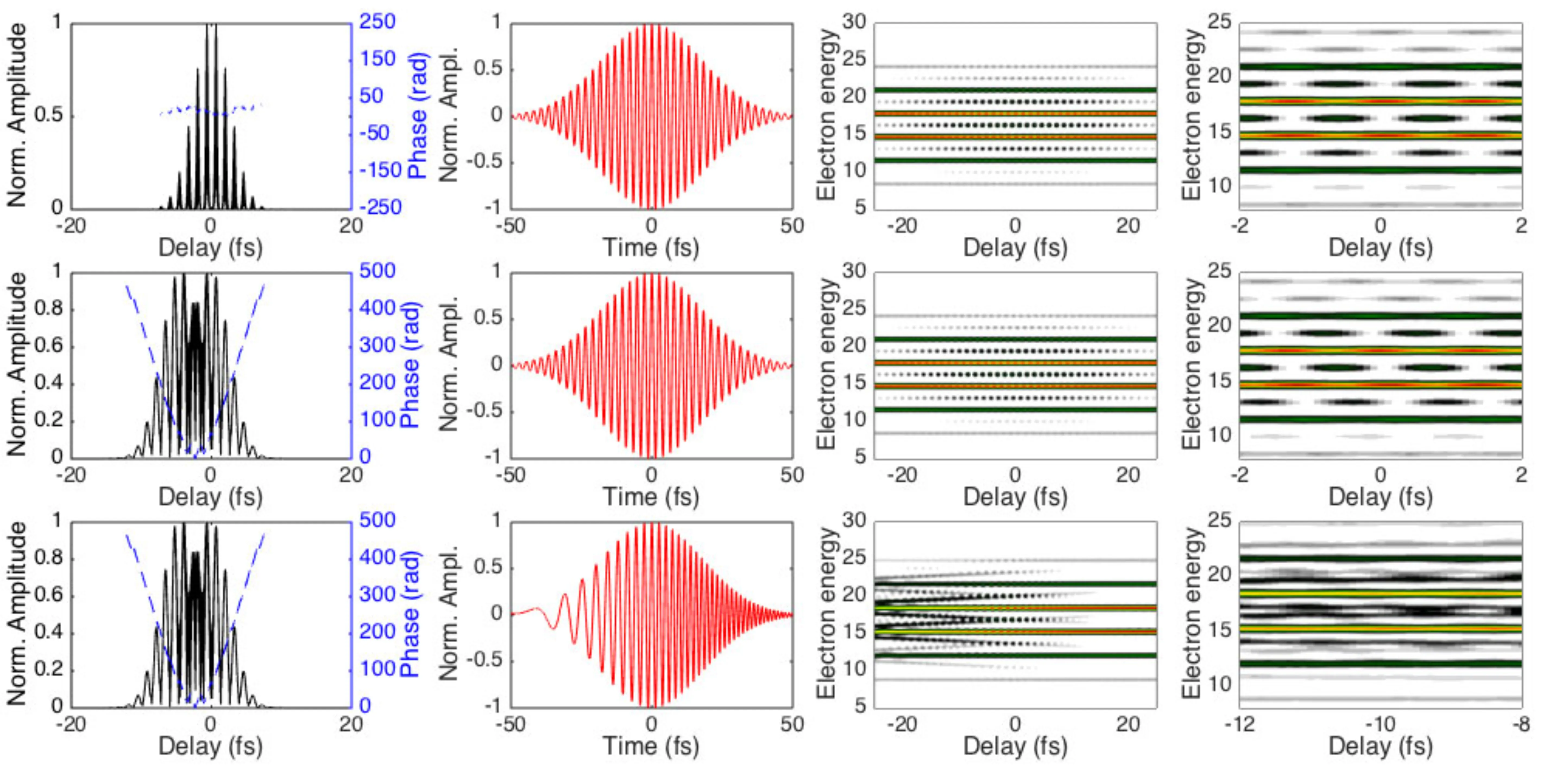
3.7 From RABBITT to Streaking Regime

This discussion is informed by concepts similar to those in the paper 'Equivalence of RABBITT and Streaking Delays'.
The transition from the conditions of a RABBITT experiment (typically using an APT and a weak IR field) to those of a streaking experiment (typically using an SAP and a strong IR field) can be conceptually demonstrated by considering the effect of successively reducing the XUV pulse (or pulse train envelope) duration. A shorter XUV pulse in the time domain implies a broader corresponding XUV excitation spectrum. This is illustrated in the following figures:

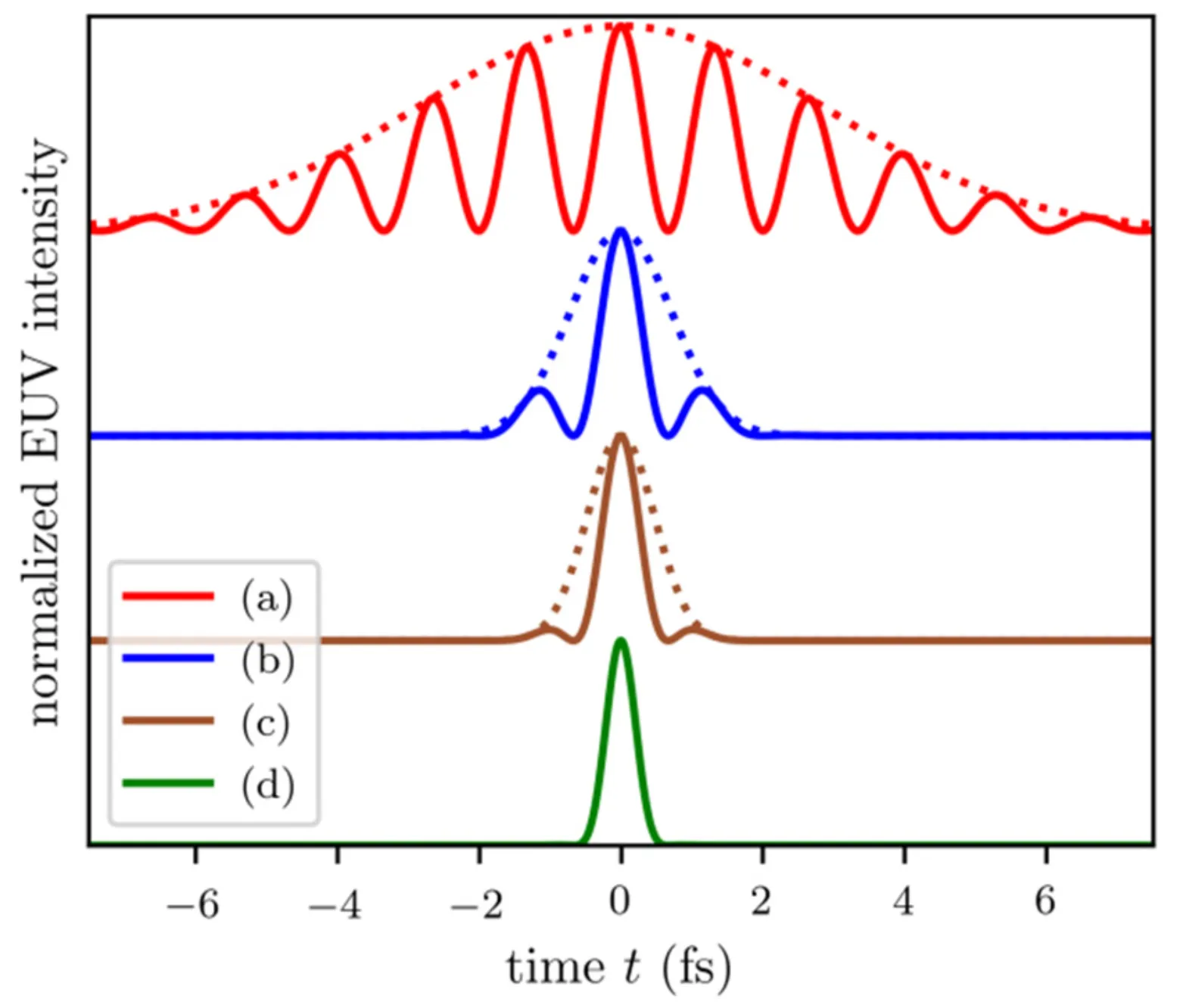
The solid line represents the normalised intensity of the XUV excitation pulses (or individual bursts within an APT envelope), corresponding to the spectra shown in the next figure. The dashed line is the overall pulse train envelope.

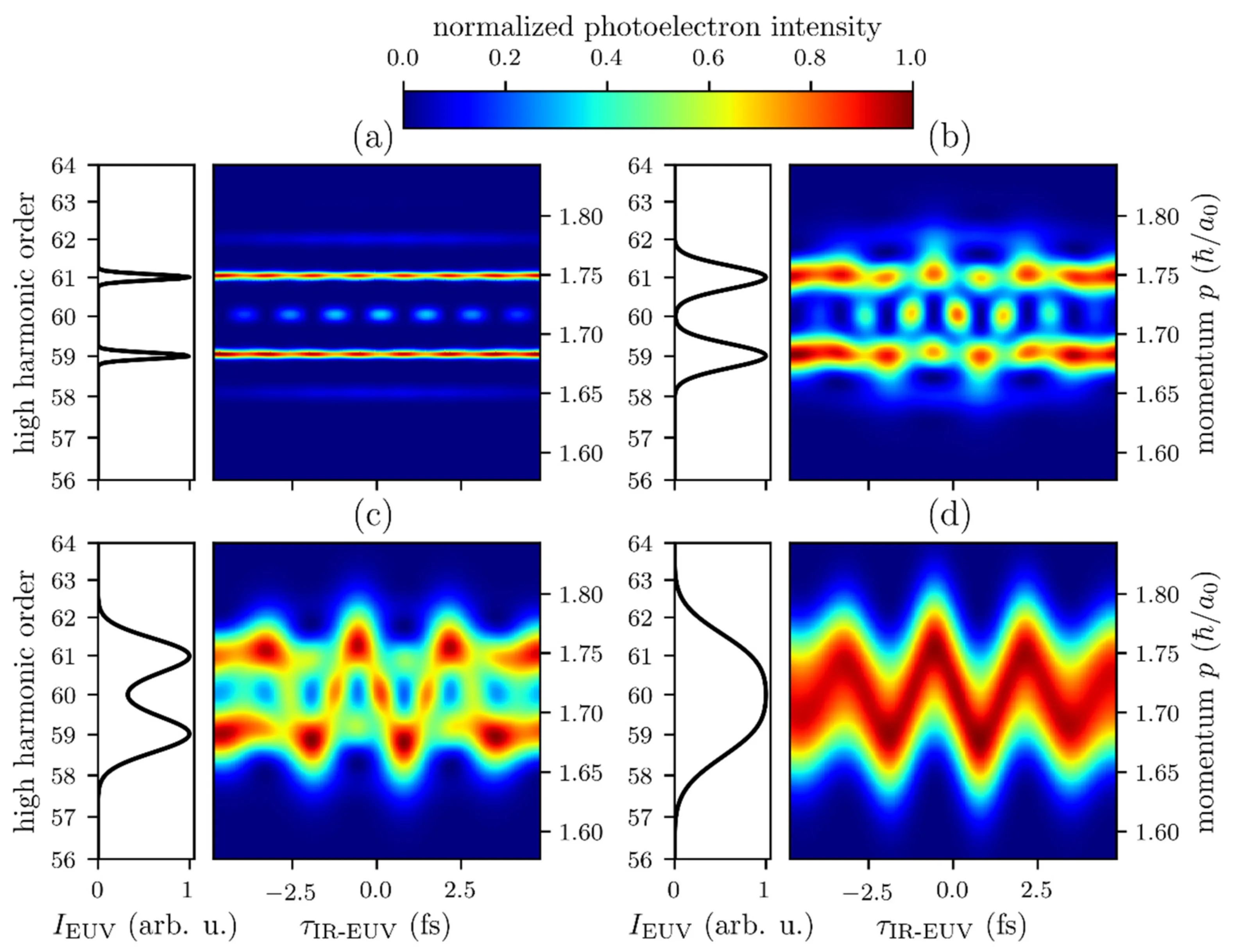
• In a 'pure' RABBITT experiment, such as shown in (a) with a relatively long XUV envelope (say, 6.7 fs FWHM for the envelope of the APT), the XUV spectrum consists of well-defined discrete harmonic lines (for instance, at the 59th and 61st harmonic orders). The interference between pathways involving adjacent harmonics gives rise to the $2{\omega }_0$ sideband oscillations.
• As the duration of the XUV excitation (either the overall APT envelope or the individual attosecond bursts if considering SAP generation) is reduced, its spectrum broadens. When the spectral width of individual harmonic orders becomes comparable to their $2{\omega }_0$ spacing, the harmonic peaks begin to merge.
• In the 'pure' streaking limit, if an isolated attosecond pulse is used (or if the APT envelope is so short that only one burst effectively interacts), the XUV spectrum becomes continuous or quasi-continuous. In figure panels (b) and (c), with progressively reduced pulse durations (implying broader spectra), the distinct sidebands characteristic of RABBITT become less prominent or merge into a broader, continuously streaked photoelectron spectrum. The main features of the APT (if still present) become more pronounced as individual, temporally shorter events. When a single attosecond pulse with a broad continuous spectrum ionises the atom, the IR field streaks the entire continuous photoelectron wavepacket, rather than modulating discrete sidebands.