Jump back to chapter selection.

Table of Contents

8.1 Fundamental Light-Matter Interaction
8.2 Einstein Coefficients and Rate Equation
8.3 Lasers
8.4 Laser Rate Equations
8.5 Experimental Parameters of Lasers
8.6 Initial Laser Dynamics
8.7 Mode Selection
8.8 Hole Burning
8.9 Pulsed Lasers - Overview
8.10 Examples of Lasers

8 Laser Fundamentals

In this chapter, the fundamental principles underlying the physics of a laser are discussed. However, before delving into the physics, let us understand what 'Laser' stands for:

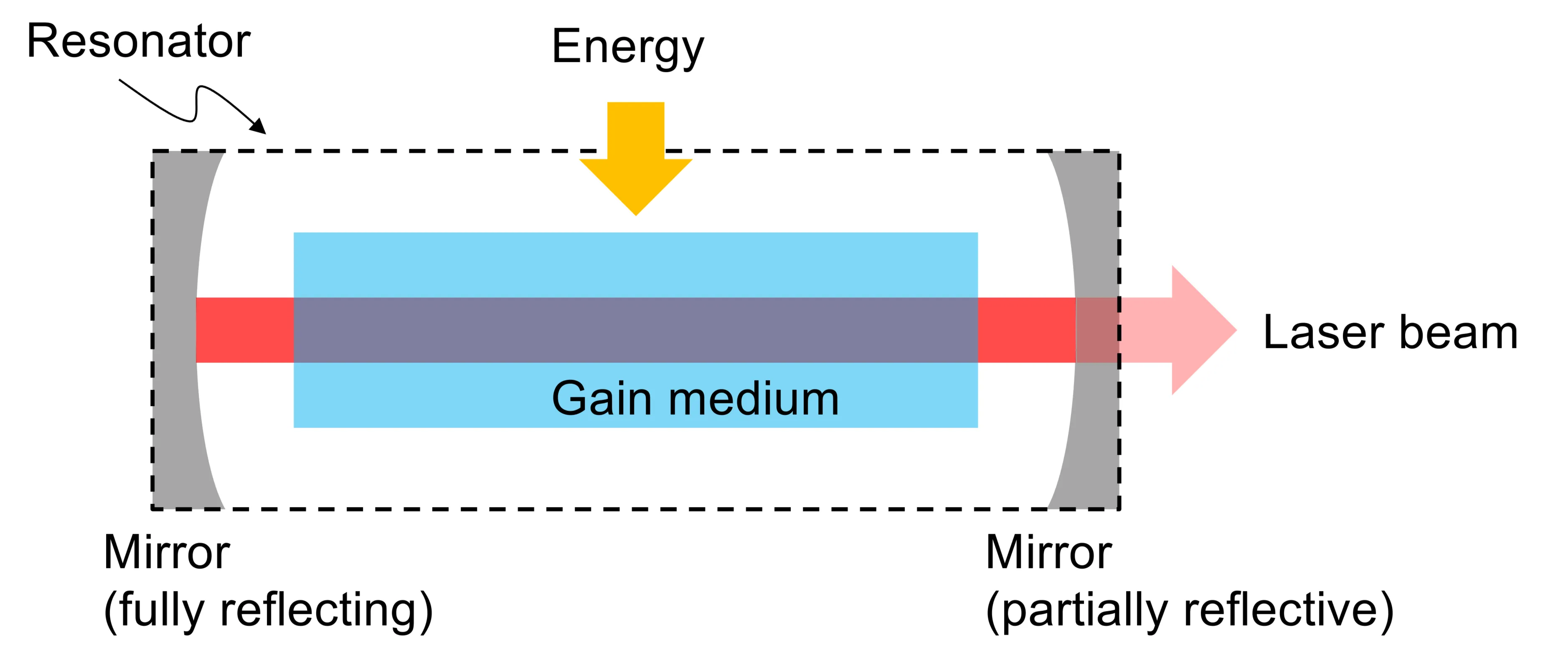
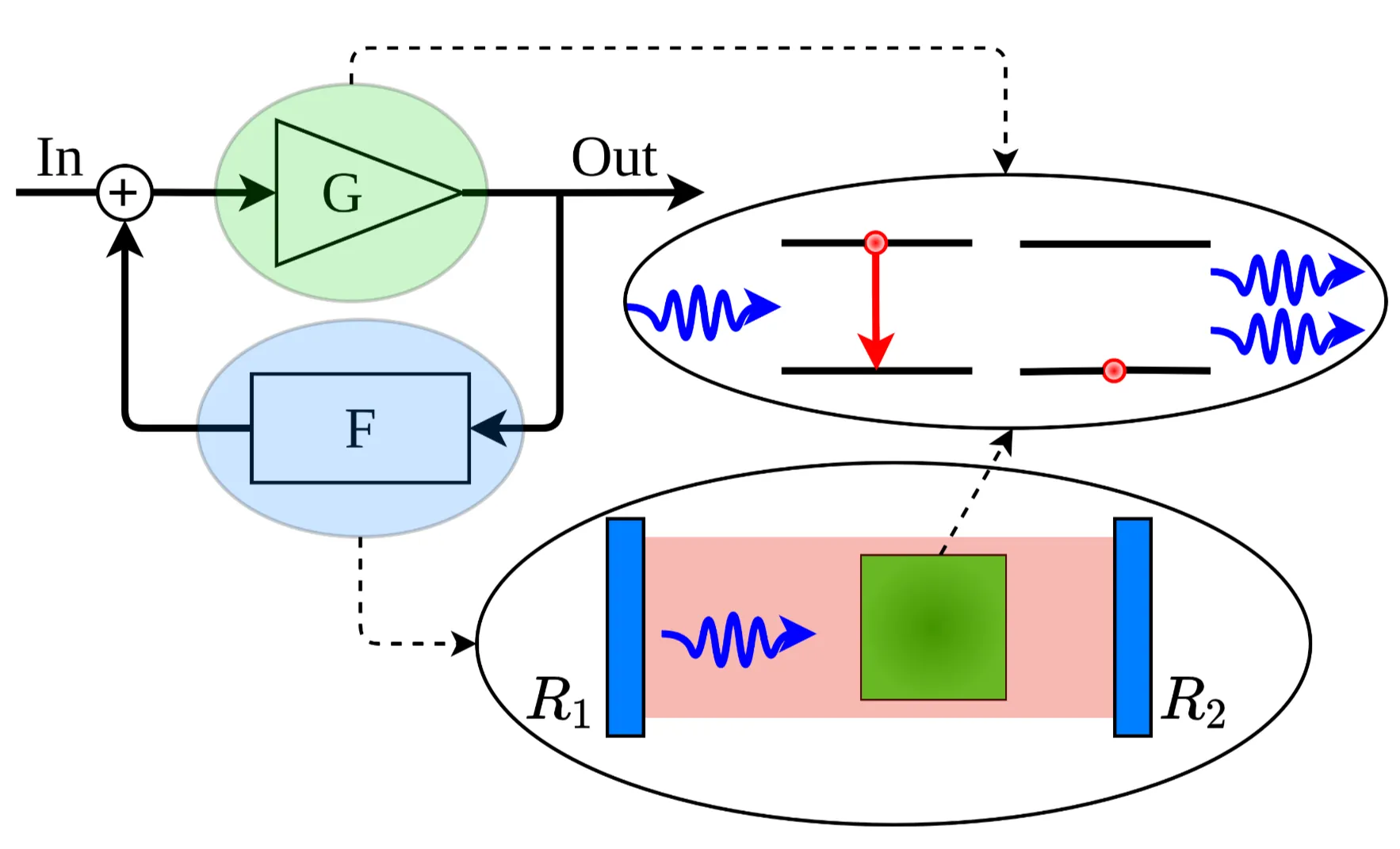
Later on, we will understand why each word in this acronym plays a crucial role for these devices to function. A laser requires, at a very basic level, an amplifying medium (called the gain medium), a feedback mechanism (typically an optical resonator), and an energy source (called the pump). For now, we will consider a laser as an optical resonator system capable of emitting coherent light. We will discuss this in more detail in section 8.3. The following figure sketches the minimum requirements that a laser needs to have, as already mentioned:

In the following section, we will first introduce Einstein coefficients and deduce from these the requirements for the gain medium.

8.1 Fundamental Light-Matter Interaction

This section aims to give a brief overview of light-matter (or photon-atom) interactions that are relevant to understanding lasers. A full treatment of this topic requires quantum electrodynamics (QED), which goes much beyond the scope of this course. First, let us consider a quantum-mechanical material, that is, a material with quantised energy levels. To keep it simple, imagine a two-level system, comprising a ground state $|1⟩$ and an excited state $|2⟩$. These states have energies $E_1$ and $E_2$, respectively, where by definition $E_1<E_2$. We will focus on interactions with photons of energy $h\nu =E_2-E_1$ (where $\nu$ is the frequency and $h$ is Planck's constant, or $\hslash \omega =E_2-E_1$ for angular frequency $\omega$). Furthermore, we will only consider the transition $|1⟩\leftrightarrow |2⟩$ to be dipole allowed. Consider the following three fundamental interaction processes:

In the following, we will assume that all these processes occur effectively instantaneously relative to other timescales of interest:

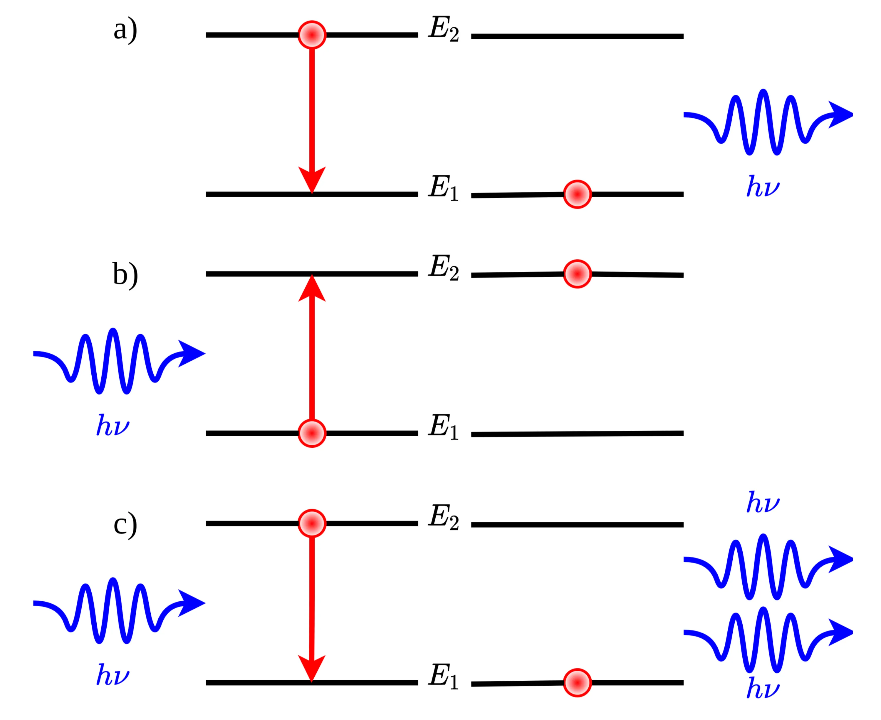
• a) Spontaneous emission: This process is independent of the presence of other photons. An atom or molecule in an excited state $|2⟩$ may spontaneously transition to the ground state $|1⟩$, releasing its excess energy as a photon with energy $h\nu =E_2-E_1$. The probability per unit time (rate) of this process for a single atom is denoted $A_{21}$.
• b) Absorption: An incoming photon of energy $h\nu$ can be absorbed by an atom in the ground state $|1⟩$, exciting it to state $|2⟩$. The probability per unit time of this process, $W_{12}^{\text{abs}}$, is proportional to the energy density of incident photons at frequency $\nu$. If $N_{ph}$ is the number of incident photons (or related to field intensity), the rate is proportional to $N_{ph}$.
• c) Stimulated emission: An incoming photon with energy $h\nu$ can interact with an atom already in the excited state $|2⟩$. This interaction can stimulate the atom to transition back to the ground state $|1⟩$, emitting a second photon. This emitted photon is identical to the incident (stimulating) photon – it has the same frequency, phase, direction of propagation, and polarisation. This property is critical for light amplification. As with absorption, the probability per unit time of stimulated emission, $W_{21}^{\text{stim}}$, is proportional to the energy density of incident photons at frequency $\nu$.

From these points, it should be clear that the rates for absorption and stimulated emission are not constant intrinsic atomic properties alone but depend on the strength of the incident electromagnetic field (related to $N_{ph}$ or energy density $\rho (\nu )$).

8.2 Einstein Coefficients and Rate Equation

Keeping the notation from above, $A_{21}$ is the rate of spontaneous emission for a single atom from level 2 to level 1 (units of ${\text{s}}^{-1}$). It is an intrinsic property of the specific atomic transition and is related to the radiative lifetime $t_{sp}$ of the excited state by:

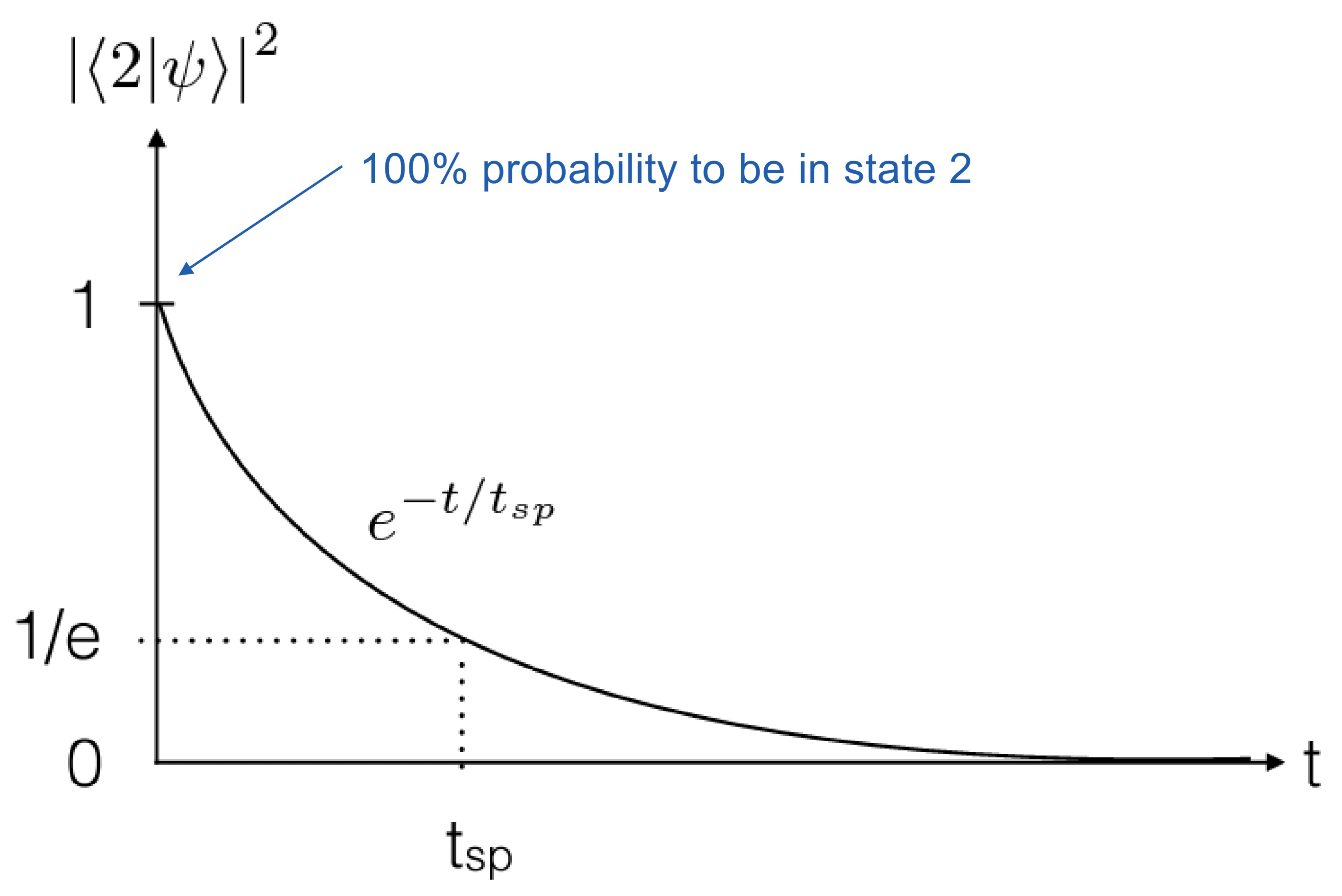
The lifetime $t_{sp}$ depends on the atom and the specific transition but not directly on the external electromagnetic field modes (though it can be modified by the local density of optical states, for instance in a cavity – the Purcell effect). Typical values for allowed atomic transitions are $t_{sp}\sim {10}^{-8}\text{s}$. The population $N_2(t)$ of an ensemble of initially excited atoms decays as $N_2(t)=N_2(0)e^{-A_{21}t}=N_2(0)e^{-t/t_{sp}}$.

Similarly, we can define the absorption rate per atom, $W_{12}$, for the transition from level 1 to level 2, and the stimulated emission rate per atom, $W_{21}$, from level 2 to level 1. These rates are proportional to the spectral energy density $\rho ({\nu }_0)$ of the electromagnetic field at the transition frequency ${\nu }_0=(E_2-E_1)/h$:

Here, $B_{12}$ and $B_{21}$ are the Einstein B coefficients for absorption and stimulated emission, respectively. These coefficients are properties of the atomic transition and are independent of the electromagnetic field strength (though they depend on the transition frequency and dipole moment). The question now is whether $A_{21},B_{12},$ and $B_{21}$ are independent of each other. The answer is no, as shown by Albert Einstein in 1917.

Consider a collection of two-level atoms inside an optical cavity, with both the atoms and the electromagnetic field inside the cavity in mutual thermal equilibrium at temperature $T$. The relative population densities of atoms in state $|1⟩$ ($N_1$) and state $|2⟩$ ($N_2$) are determined by the Boltzmann distribution:

where $g_1,g_2$ are the degeneracies of the levels, often assumed $g_1=g_2=1$ for simplicity.
The rate of change of $N_2$ is the sum of rates for all processes:

For population densities $N_1,N_2$:

In thermal equilibrium, $d{N}_2/dt=0$, so:

Solving for $\rho ({\nu }_0)$:

Substituting $N_1/N_2=(g_1/g_2)e^{h{\nu }_0/k_{B}T}$:

This expression for $\rho ({\nu }_0)$ must be identical to Planck's blackbody radiation law for spectral energy density:

(where $n$ is the refractive index of the medium, $n\approx 1$ if cavity is near vacuum).
Comparing these two expressions for $\rho ({\nu }_0)$ yields the Einstein relations:

If $g_1=g_2$ (non-degenerate levels or equally degenerate), then $B_{12}=B_{21}\equiv B$. The Einstein A and B coefficients are then related by:

This allows relating the probabilities (rates per atom per unit energy density) for absorption and stimulated emission to the probability (rate per atom) for spontaneous emission. The derivation also shows a fundamental symmetry between stimulated emission and absorption ($g_1{B}_{12}=g_2{B}_{21}$). Without stimulated emission, thermal equilibrium would not be consistent with Planck's law.
Although derived assuming thermal equilibrium, these relations between $A_{21},B_{12},B_{21}$ are fundamental properties of the atomic system and hold universally, irrespective of whether the system is in thermal equilibrium. The coefficients $A$ and $B$ depend on the type of atom and specific transition involved. The local electromagnetic environment (for instance, a resonant cavity) can modify the spontaneous emission rate $A_{21}$ (Purcell effect), which would then also modify $B_{12}$ and $B_{21}$ through these relations.

8.2.1 Transition Width

The energy difference between two states is $\hslash {\omega }_0=E_2-E_1$. Ideally, one might expect transitions to occur at this exact frequency, resulting in an infinitely narrow spectral line. However, this is not observed in realistic systems:

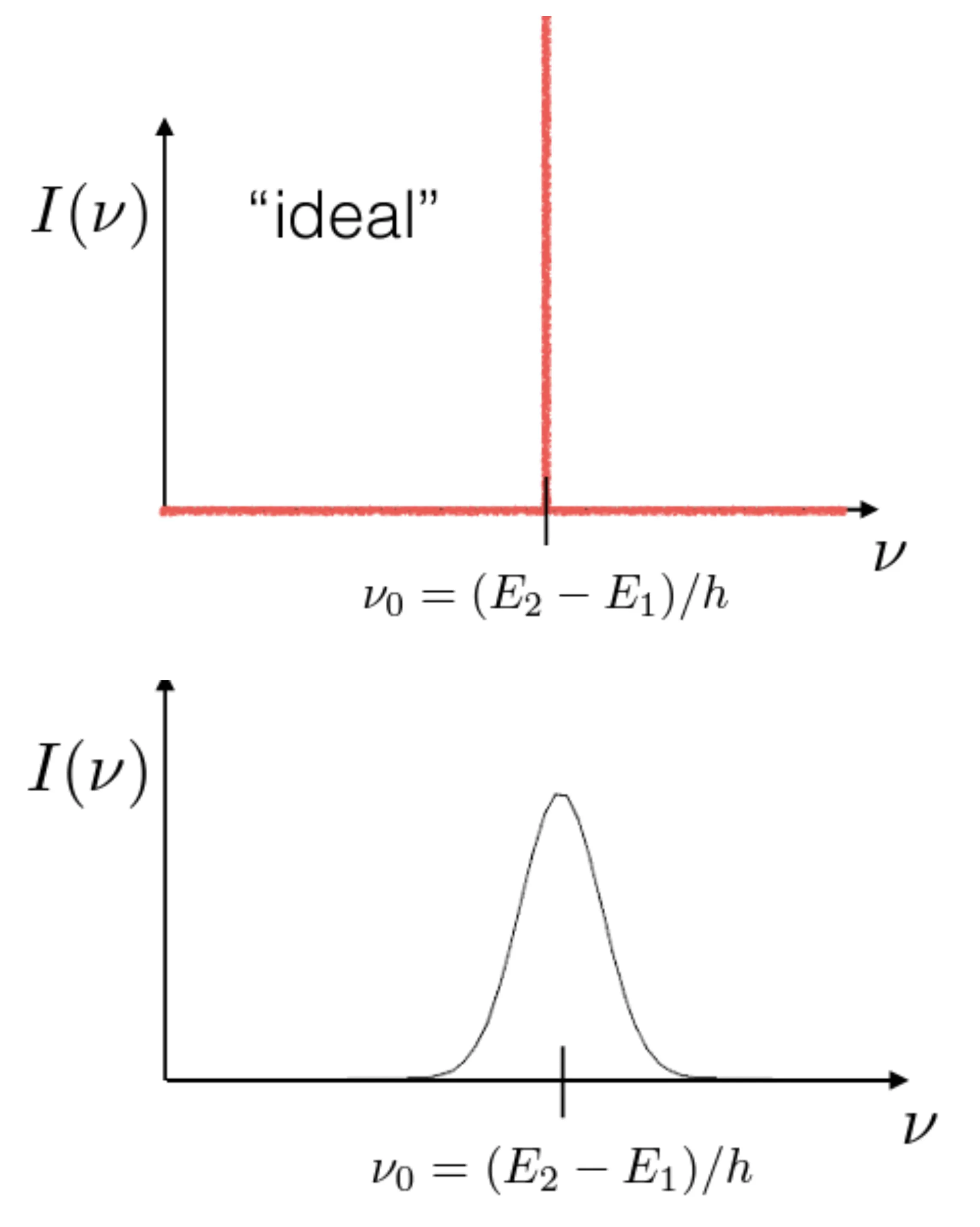
Real transitions always have a finite width in energy (and thus frequency). This broadening occurs even with an ideal spectrometer possessing arbitrarily high spectral resolution. Several physical effects contribute to this broadening.

8.2.2 Homogeneous vs Inhomogeneous Broadening

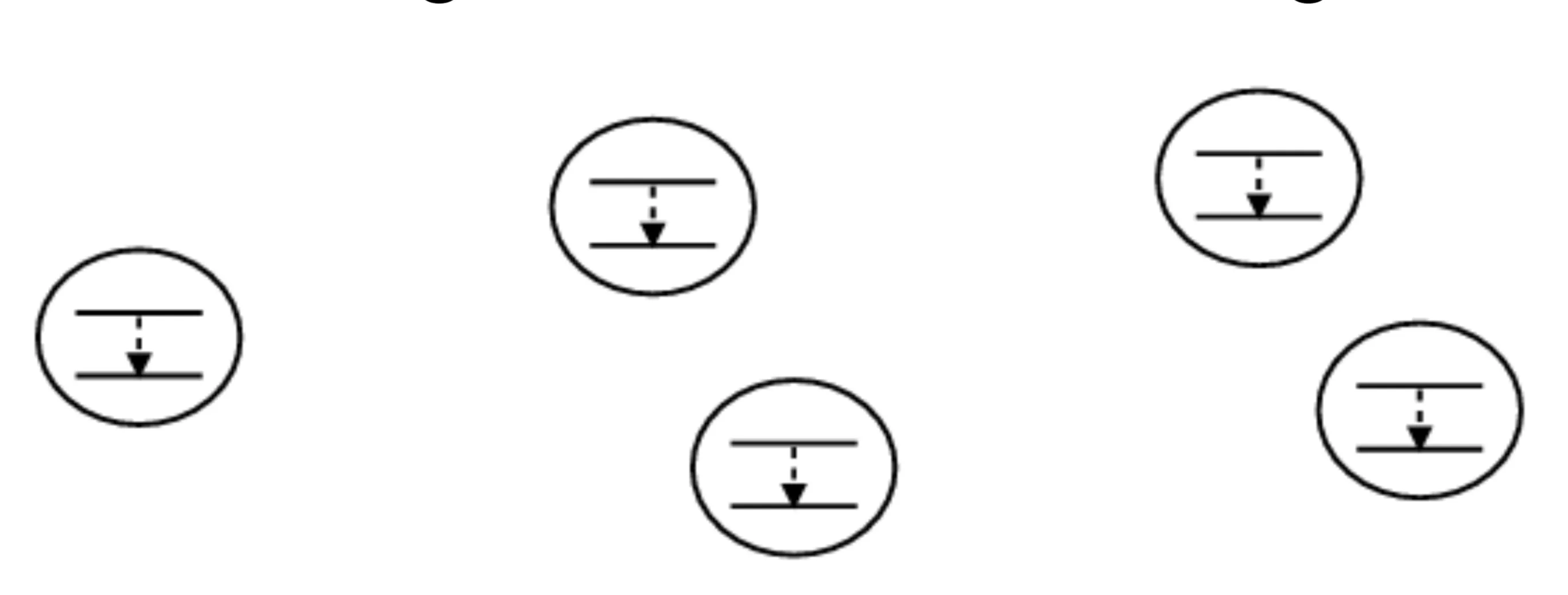
Homogeneous broadening occurs when the broadening mechanism affects all atoms (or molecules) in the ensemble in an identical way. Each atom effectively has the same resonance frequency and the same broadened lineshape.

Examples include:

• Lifetime broadening (Natural broadening): Arises from the finite lifetime $t_{sp}$ of the excited state due to spontaneous emission, dictated by the energy-time uncertainty principle ($\mathrm{\Delta }E\mathrm{\Delta }t\ge \hslash /2$).
• Collision broadening (Pressure broadening): Collisions between atoms interrupt the emission process, effectively shortening the coherence time of the emitted radiation. In a dense gas or liquid, all atoms experience similar average collision rates.

Inhomogeneous broadening occurs when different atoms in the ensemble experience slightly different local environments or conditions, leading to a distribution of individual resonance frequencies. The overall observed spectral line is the sum of many narrower lines, each slightly shifted.

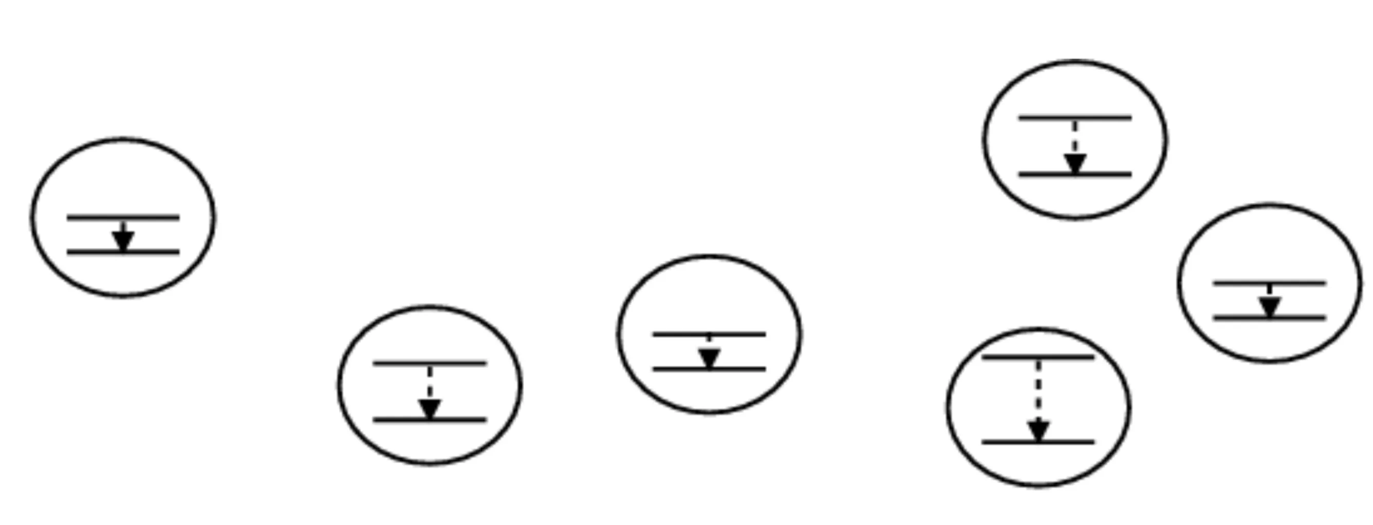
An important example is Doppler broadening in gases, where atoms moving with different velocities relative to an observer (or a detector) exhibit different apparent transition frequencies due to the Doppler effect. Another example is broadening in solids due to variations in the local crystal field experienced by different active ions.

Let us consider lifetime broadening again. The intensity of light $I(t)$ emitted by an ensemble of atoms, initially excited at $t=0$ and then decaying by spontaneous emission with a lifetime $t_{sp}$, is proportional to $e^{-t/t_{sp}}$ for $t>0$. The corresponding electric field $E(t)$ of the emitted wave behaves as:

(The factor of $1/2$ in the exponential decay of the field amplitude ensures the intensity decays as $e^{-t/t_{sp}}$).
Fourier transforming this decaying sinusoidal field yields a spectral intensity profile $I(\nu )$ that is Lorentzian:

where $\mathrm{\Delta }{\nu }_L=A_{21}/(2\pi )=1/(2\pi t_{sp})$ is the FWHM linewidth of this lifetime-broadened (natural) lineshape.

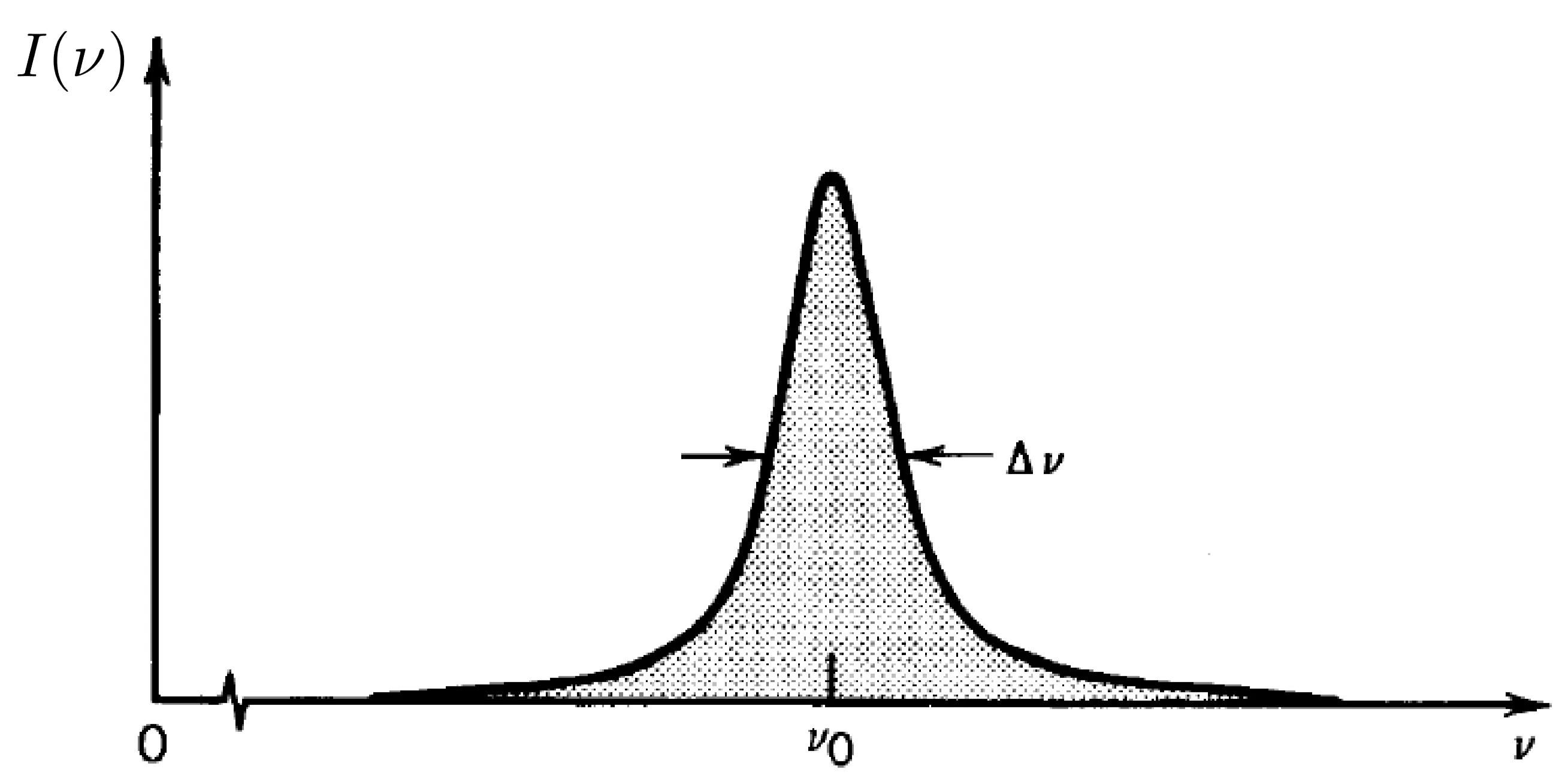
This corresponds to an ensemble of atoms where each atom emits light with this characteristic spectral profile. The normalised lineshape function $g(\nu )$ associated with a Lorentzian profile is:

Its general properties are $I(\nu )\sim g(\nu )$ (at peak) and ${\int }_{-\mathrm{\infty }}^{\mathrm{\infty }}g(\nu )d\nu =1$. Generally, homogeneous broadening processes result in Lorentzian lineshapes.
In contrast, if a Doppler broadened spectrum consists of a statistical distribution of individual, shifted (but perhaps still lifetime-broadened) Lorentzian spectra, the overall observed lineshape for inhomogeneous broadening is often Gaussian.

8.2.3 Absorption Cross-Section

The absorption cross-section $\sigma (\nu )$ quantifies the effective area an atom presents to incident photons of frequency $\nu$ for absorption. The number of photons $d{n}_{\text{abs}}$ absorbed from a single mode $j$ by one atom in time $dt$ is $d{P}_{12,j}^{\text{abs}}=W_{12,j}dt$. This can also be expressed using the photon flux ${\varphi }_j$ (photons per unit area per unit time) in mode $j$:

The absorption cross-section $\sigma (\nu )$ is related to the Einstein B coefficient and also to the A coefficient and the lineshape function $g(\nu )$:

where ${\lambda }_0$ is the vacuum wavelength of the transition, $n$ is the refractive index of the medium, and $g(\nu )$ is the normalised lineshape function ($\int g(\nu )d\nu =1$). The same cross-section (with appropriate level degeneracies $g_1,g_2$) applies to stimulated emission: ${\sigma }_{em}(\nu )=(g_1/g_2){\sigma }_{abs}(\nu )$.

8.3 Lasers

Let us now return to achieving a functioning laser. For simplicity, we will consider a laser cavity designed to amplify light primarily in a small number of resonant modes:

8.3.1 Population Inversion, Lasing Conditions and Gain

The ultimate goal of a laser is to increase the photon number $\overline{n}$ (average number of photons in a cavity mode) through net stimulated emission. In a two-level system, the rate of change of $\overline{n}$ within a single cavity mode due to interaction with atoms having populations $N_1$ (ground) and $N_2$ (excited) is:

Using Einstein coefficients, this can be written as (ignoring cavity losses for now):

where $A_{21}^{\text{mode}}$ is the rate of spontaneous emission into the specific lasing mode (often proportional to $A_{21}$).
For net amplification by stimulated emission, we need $N_2{B}_{21}\rho ({\nu }_0)>N_1{B}_{12}\rho ({\nu }_0)$.
Using $g_1{B}_{12}=g_2{B}_{21}$, this condition becomes $N_2(g_1/g_2)>N_1$, or for $g_1=g_2$, simply $N_2>N_1$.
This condition, $N_2>N_1$ (or more generally $N_2/g_2>N_1/g_1$), is called population inversion. It means there are more atoms in the excited state (per degeneracy) than in the lower state involved in the lasing transition. Population inversion is a non-equilibrium condition, strongly contrasting with Boltzmann statistics for thermal equilibrium, where $N_2/g_2<N_1/g_1$ always holds. Achieving population inversion requires externally supplying energy to the atoms. This process is called pumping and can be done optically (using another light source like a flashlamp or another laser) or electrically (using an electrical discharge or current injection).

Another requirement for lasing is feedback. To ensure that stimulated emission dominates spontaneous emission and to build up a substantial photon number in a specific mode, the emitted photons must be confined and made to pass through the gain medium multiple times. This is achieved by placing the gain medium within an optical resonator (cavity), typically formed by two mirrors. The resonator selectively enhances specific frequencies (its resonant modes) and provides the feedback, greatly increasing $\rho ({\nu }_0)$ within these modes and thus boosting the stimulated emission rate.

The notion of gain quantifies the amplification. If a photon flux $\varphi$ (or intensity $I$) propagates through an inverted medium, its rate of increase with distance $z$ is:

Here, $\gamma (\nu )$ (or $g_I(\nu )$) is the gain coefficient (per unit length). It is proportional to the population inversion $N=N_2-(g_2/g_1)N_1$ and the emission cross-section ${\sigma }_{em}(\nu )$: $\gamma (\nu )=N{\sigma }_{em}(\nu )$ (if $N$ is inversion density $(N_2/g_2-N_1/g_1)g_2$).
The total gain $G(\nu )$ after passing through a gain medium of length $d$ is $G(\nu )=e^{\gamma (\nu )d}$. It depends strongly on the amount of population inversion.

Thus, schematically a laser involves pumping to achieve population inversion in a gain medium, which is placed inside an optical resonator to provide feedback and mode selection:

The feedback also provides narrow spectral filtering due to the cavity resonances.

8.3.2 Achieving Population Inversion

As mentioned, pumping the system from state $|1⟩$ to state $|2⟩$ and expecting lasing on the same $|2⟩\to |1⟩$ transition (a pure two-level system) does not lead to population inversion. The steady-state rate balance equation, $W_{12}^{\text{pump}}{N}_1=A_{21}{N}_2+W_{21}^{\text{stim}}{N}_2$, where $W_{12}^{\text{pump}}$ is the pumping rate from 1 to 2, and $W_{21}^{\text{stim}}$ is the stimulated emission rate from 2 to 1 due to the generated photons, shows this. If $g_1{B}_{12}=g_2{B}_{21}$, then $W_{12}^{\text{stim}}=(g_2/g_1)W_{21}^{\text{stim}}$. Even with very strong pumping, the best one can achieve is $N_2/g_2\approx N_1/g_1$ (saturation), but not $N_2/g_2>N_1/g_1$. Therefore, population inversion is not possible in a simple two-level system when pumped and lased on the same transition. This necessitates using systems with at least three or four energy levels.

The small-signal gain coefficient ${\gamma }_0(\nu )$ is the maximum gain achieved when the population inversion $N_0$ is at its maximum (for instance, in the absence of photons in the cavity to cause stimulated emission, $I\approx 0$): ${\gamma }_0(\nu )=N_0{\sigma }_{em}(\nu )$.

8.3.3 Three-Level Laser Systems

Since population inversion is unobtainable in an ideal two-level system pumped on the lasing transition, we consider systems with more levels. A three-level system is the minimum required for achieving inversion.

The general layout is:

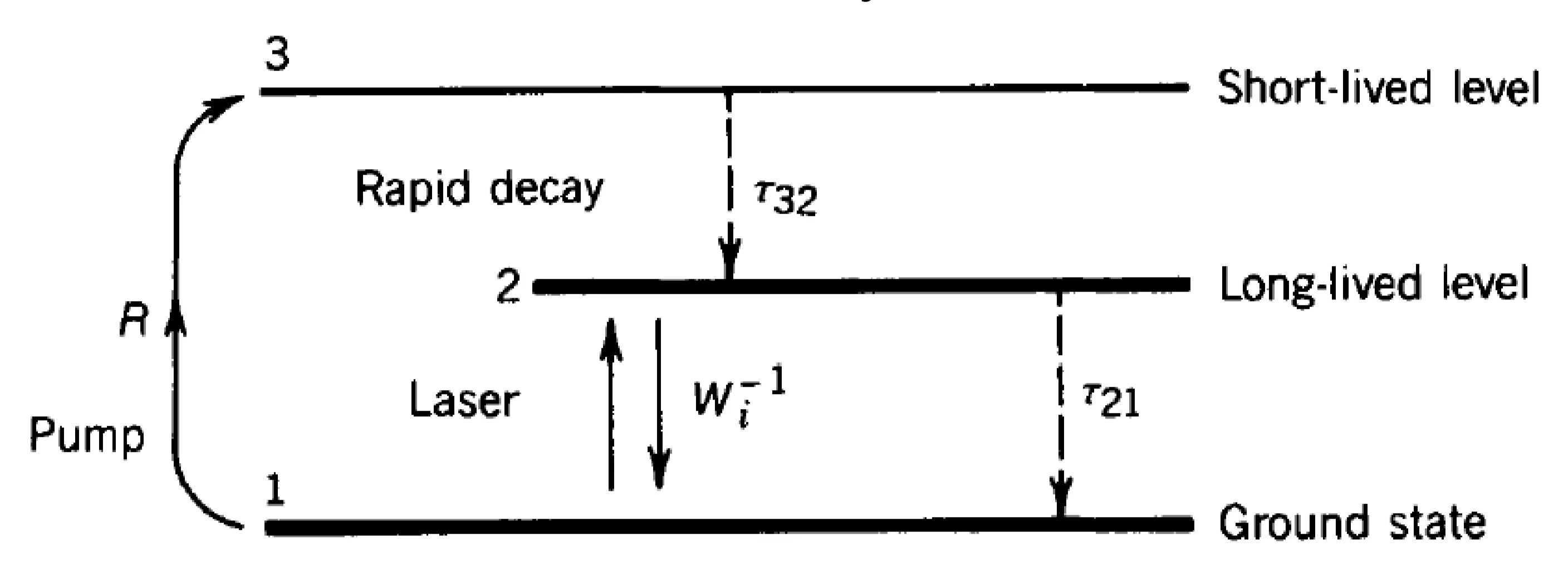
Atoms are pumped from the ground state $|1⟩$ to a higher energy level $|3⟩$. This level $|3⟩$ is typically a broad absorption band and is short-lived, with atoms rapidly decaying (often non-radiatively, lifetime ${\tau }_{32}$) to an intermediate metastable level $|2⟩$. The lasing transition then occurs between level $|2⟩$ and the ground state $|1⟩$. The lifetime of level $|2⟩$ due to spontaneous emission to state $|1⟩$ is ${\tau }_{21}$, which needs to be long to allow population to accumulate in $|2⟩$.
The rate equations (assuming $N_3$ is small due to fast decay ${\tau }_{32}\ll {\tau }_{21}$, so pumped atoms quickly arrive in state $|2⟩$ at a rate $R_p\approx W_p{N}_1$) become approximately:

where $N_1+N_2\approx N_{\text{total}}$ (total active atom density) and $W_i=B\rho ({\nu }_0)$ is the stimulated transition rate for the $|2⟩\leftrightarrow |1⟩$ transition.
Solving for steady-state ($d{N}_2/dt=0,d{N}_1/dt=0$), the population inversion $N=N_2-N_1$ can be found.
Achieving inversion ($N_2>N_1$) in a three-level system is possible, but requires strong pumping because the lower laser level is the ground state, which is heavily populated at thermal equilibrium. More than half of the total atoms must be pumped out of the ground state into the excited state $|2⟩$ to achieve $N_2>N_1$. This makes three-level lasers generally less efficient and require higher pump powers. Additionally, reabsorption of laser photons by ground state atoms can be a significant loss.

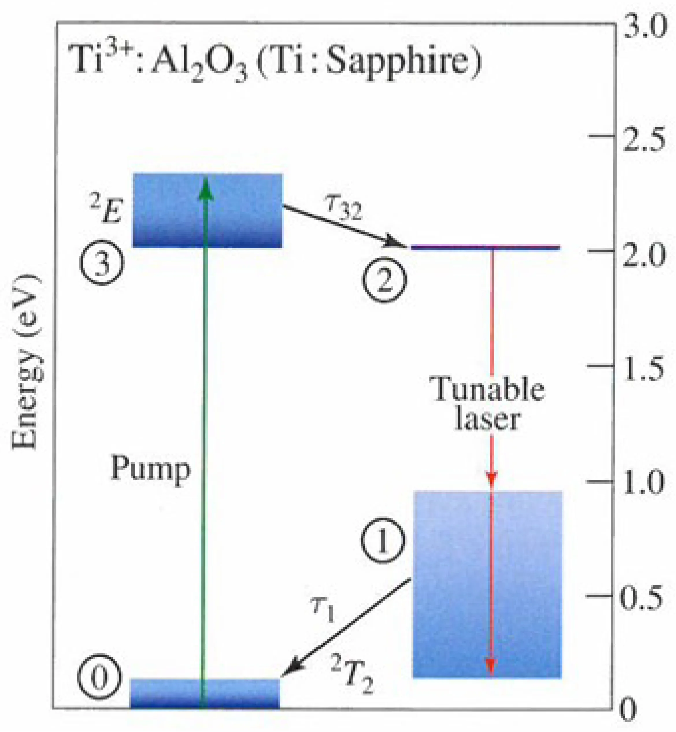
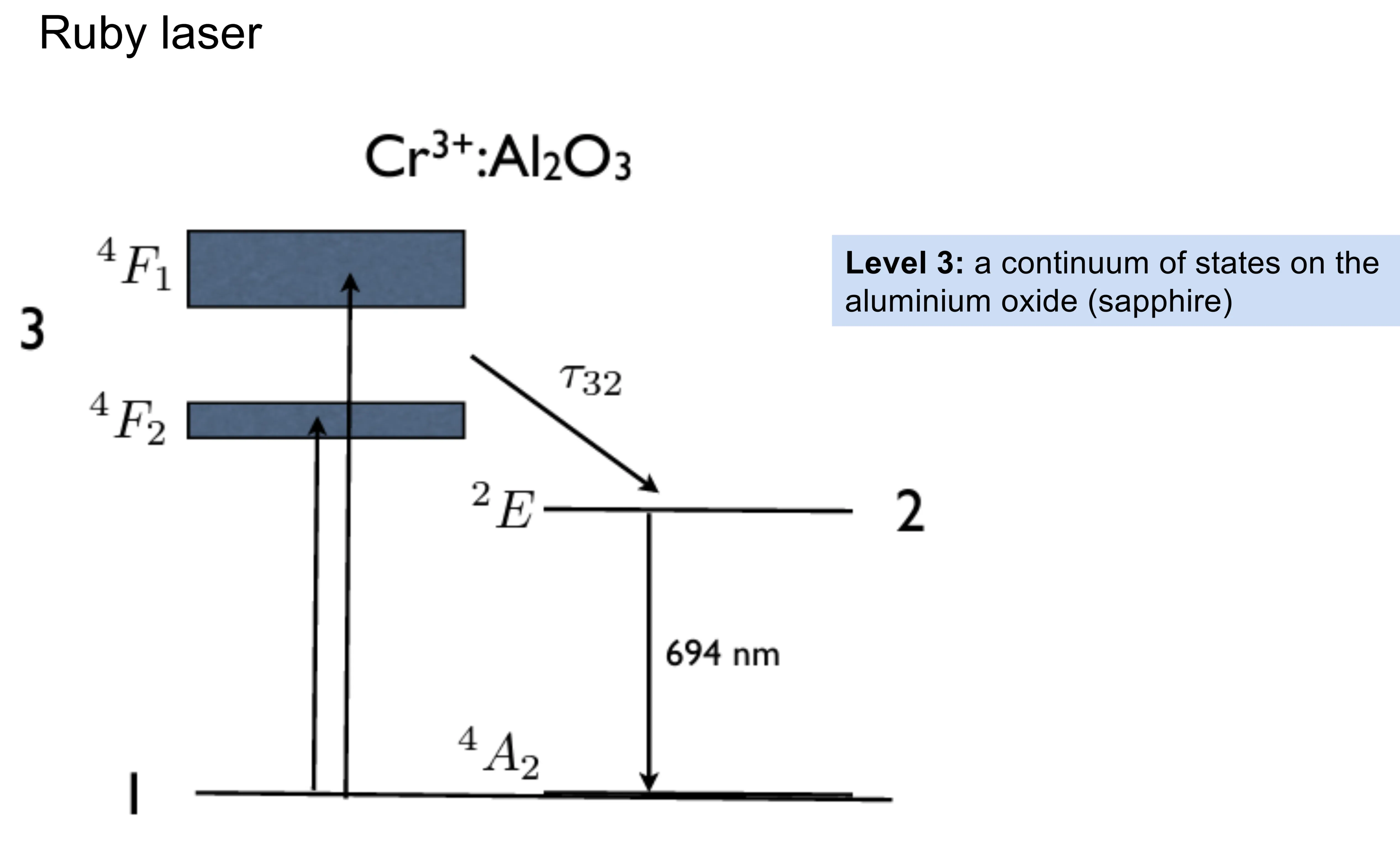
The first laser, the ruby laser (${\text{Cr}}^{3+}$ in ${\text{Al}}_2{\text{O}}_3$), was a three-level system:

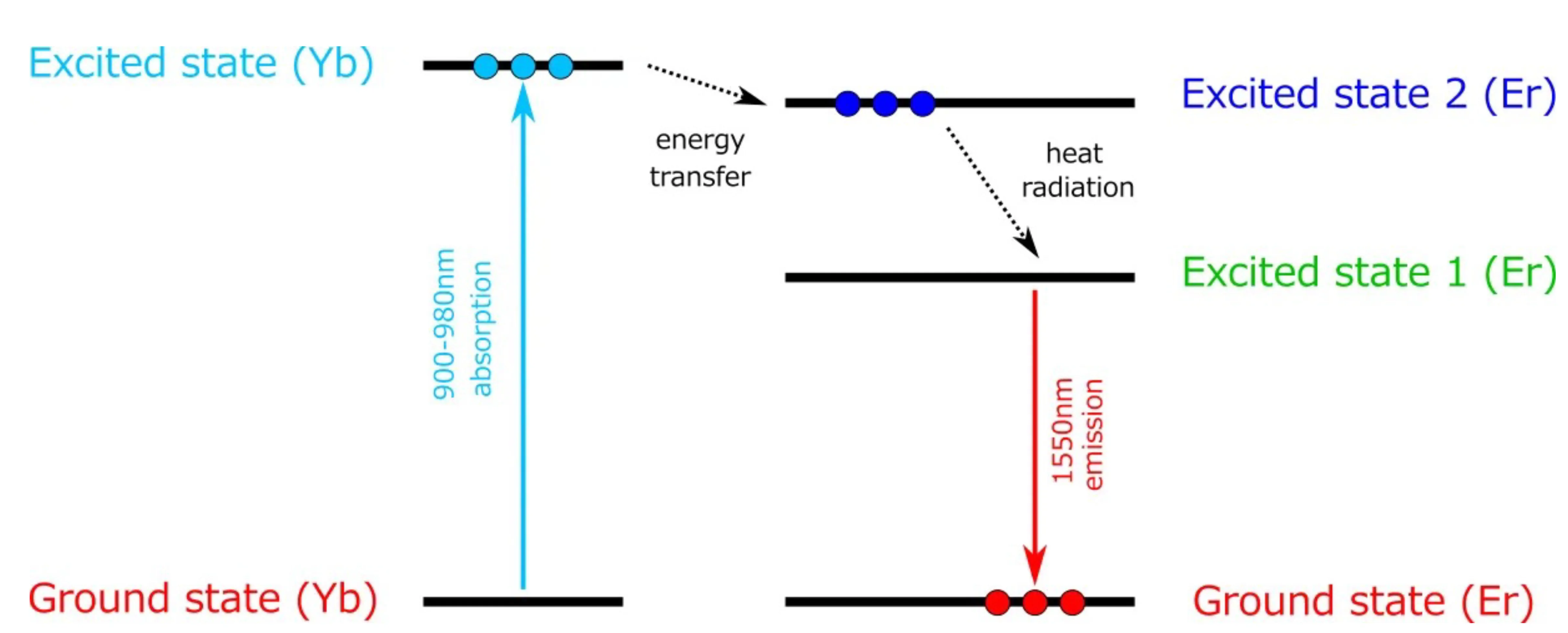
Erbium-doped silica fibre amplifiers/lasers can also operate on a quasi-three-level scheme depending on the wavelength.

Ytterbium-doped YAG ($\text{Yb:YAG}$) is another important gain medium that can operate as a quasi-three-level system (the lower laser level is very close to the ground state).

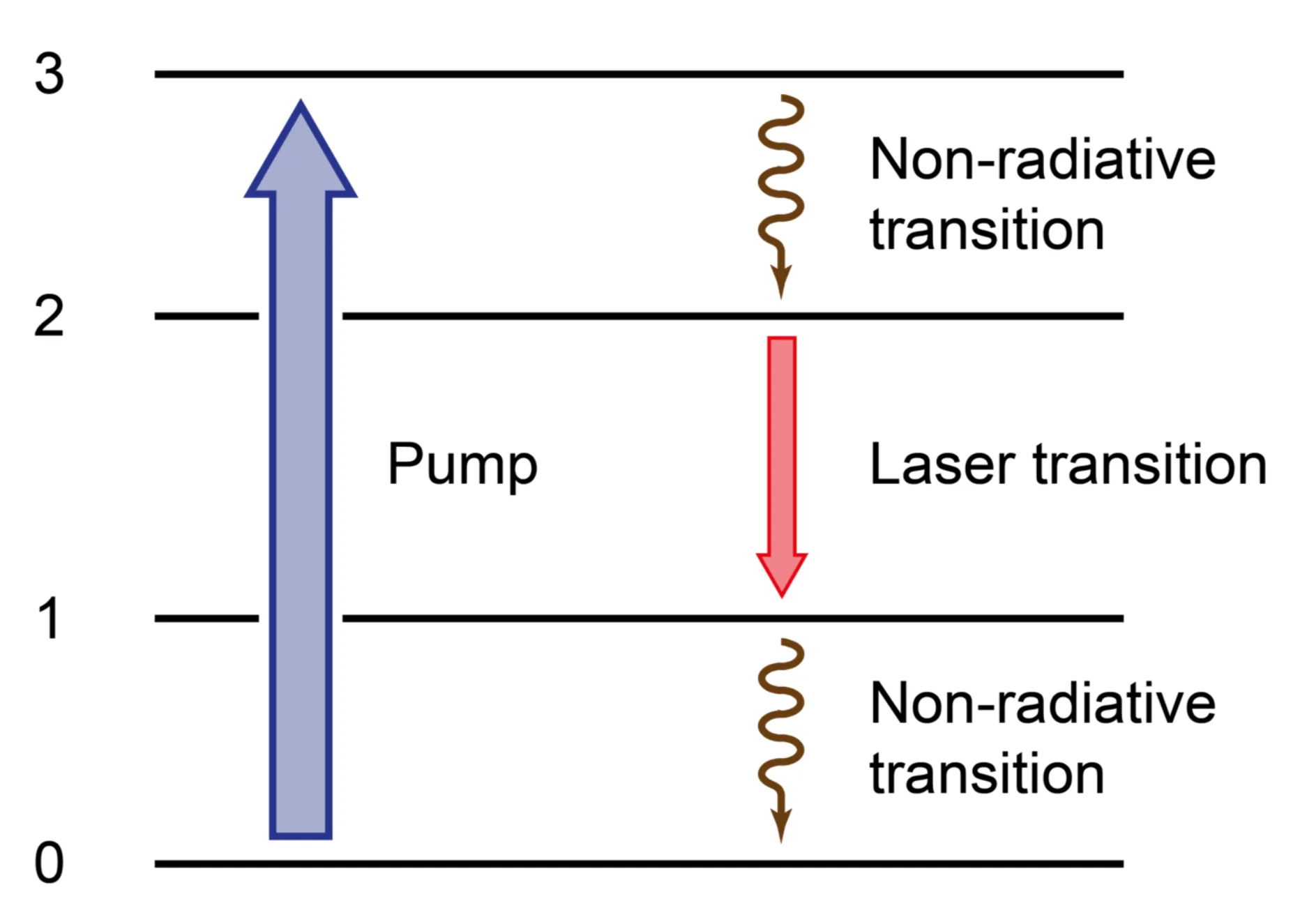
8.3.4 Four-Level System

The challenges of high pump thresholds in three-level systems are largely overcome in a four-level system:

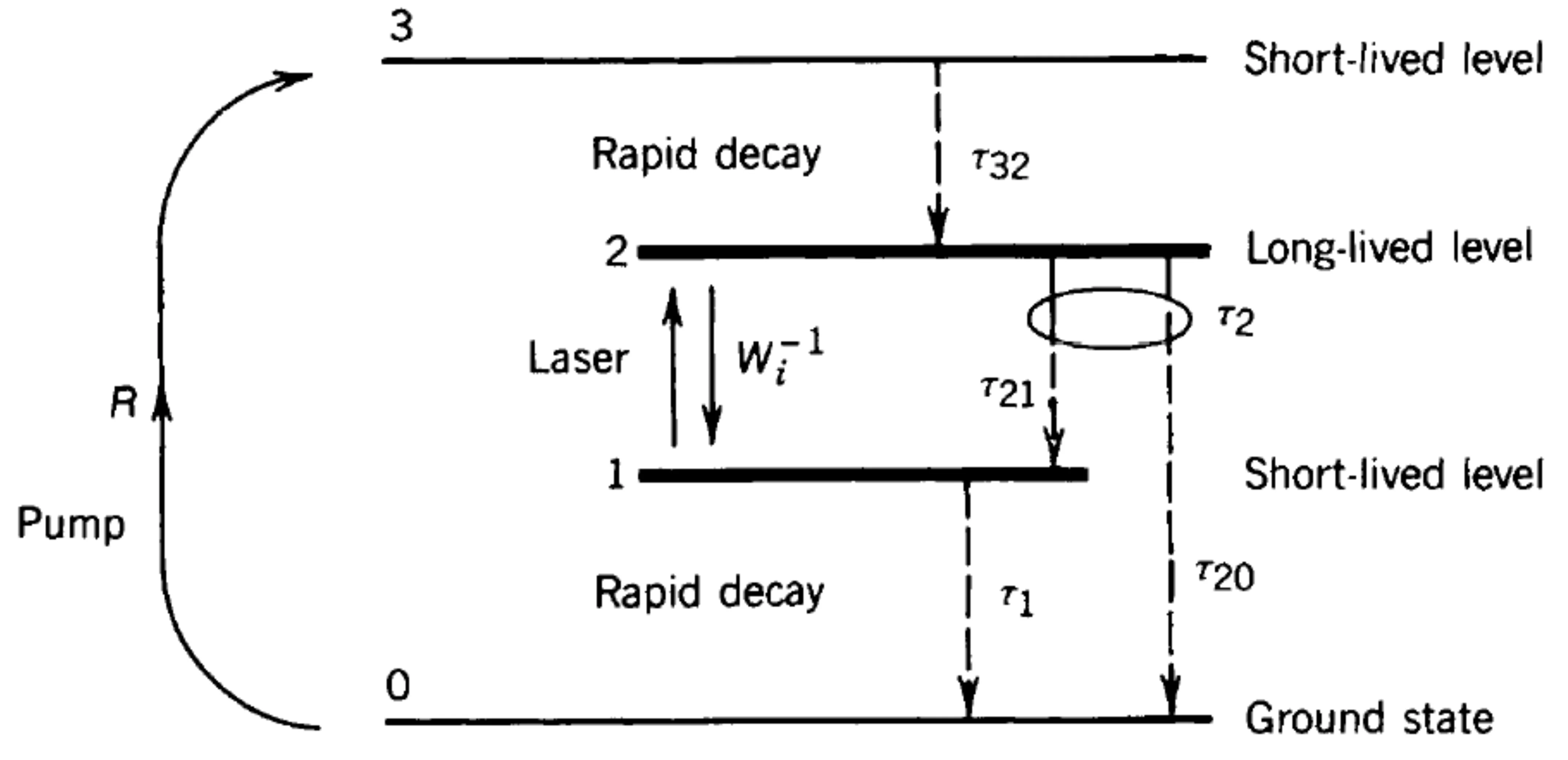
Here, atoms are pumped from the ground state $|0⟩$ to a higher pump band $|3⟩$. They rapidly decay from $|3⟩$ to the upper laser level $|2⟩$ (metastable). The lasing transition occurs between $|2⟩$ and a lower laser level $|1⟩$. Crucially, level $|1⟩$ is above the ground state $|0⟩$ and rapidly depopulates to the ground state (lifetime ${\tau }_{10}$ is very short).
This rapid depopulation of the lower laser level $|1⟩$ ensures that its population $N_1$ remains very small. Thus, population inversion ($N_2>N_1$) between levels $|2⟩$ and $|1⟩$ can be achieved with much lower pumping rates than in a three-level system, as $N_1\approx 0$.
The rate equations simplify under these assumptions (${\tau }_{32}\to 0$, ${\tau }_{10}\to 0$). The steady-state inversion $N=N_2-N_1\approx N_2$ is given by similar forms as for the three-level system but with parameters that make $N>0$ much easier to achieve for a given pump rate $W_p$.
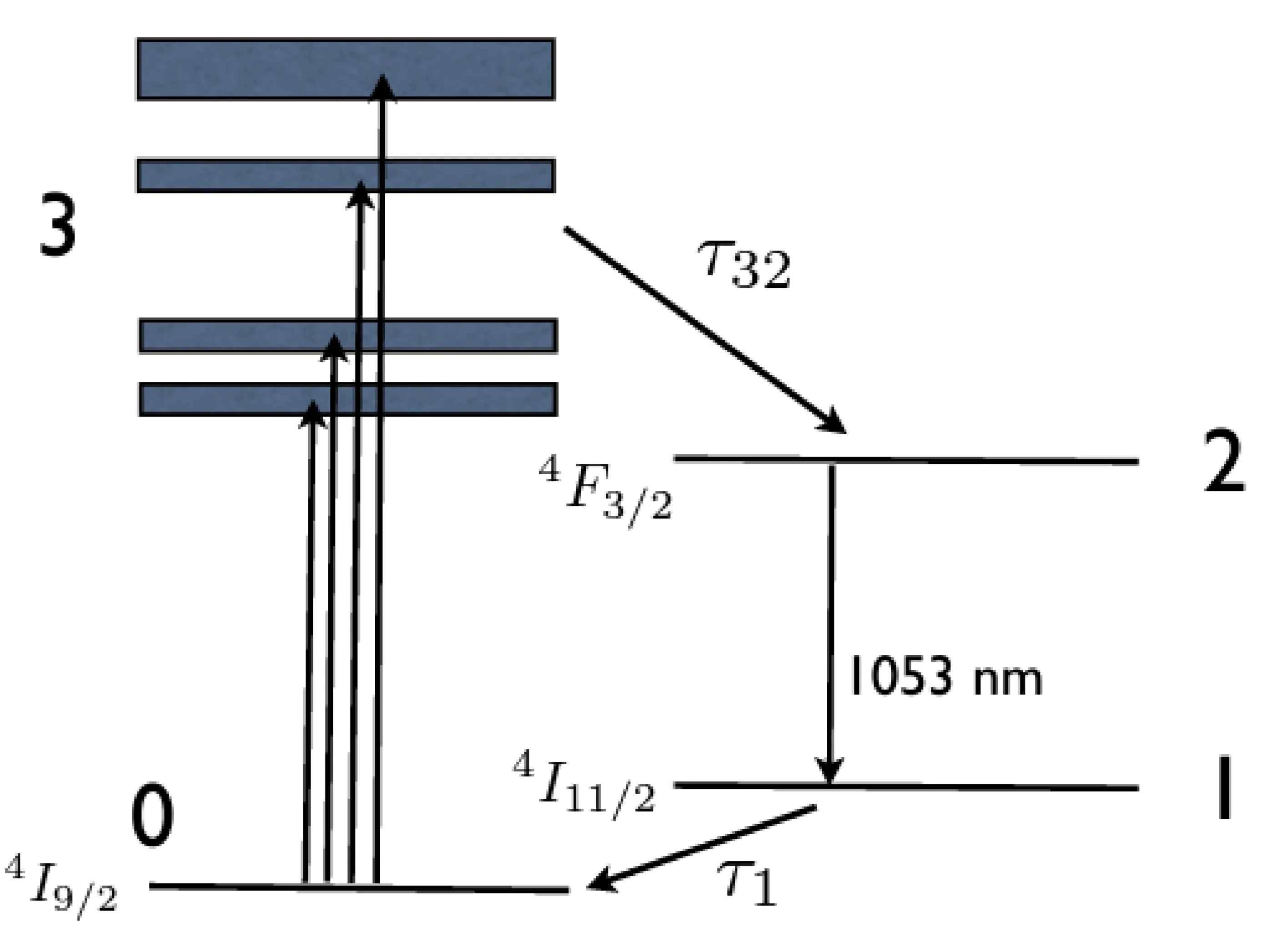
One example of a four-level laser system is Nd:YAG or Nd:glass (neodymium-doped YAG crystal or glass), widely used in high-power applications.

8.3.5 Pumping Schemes

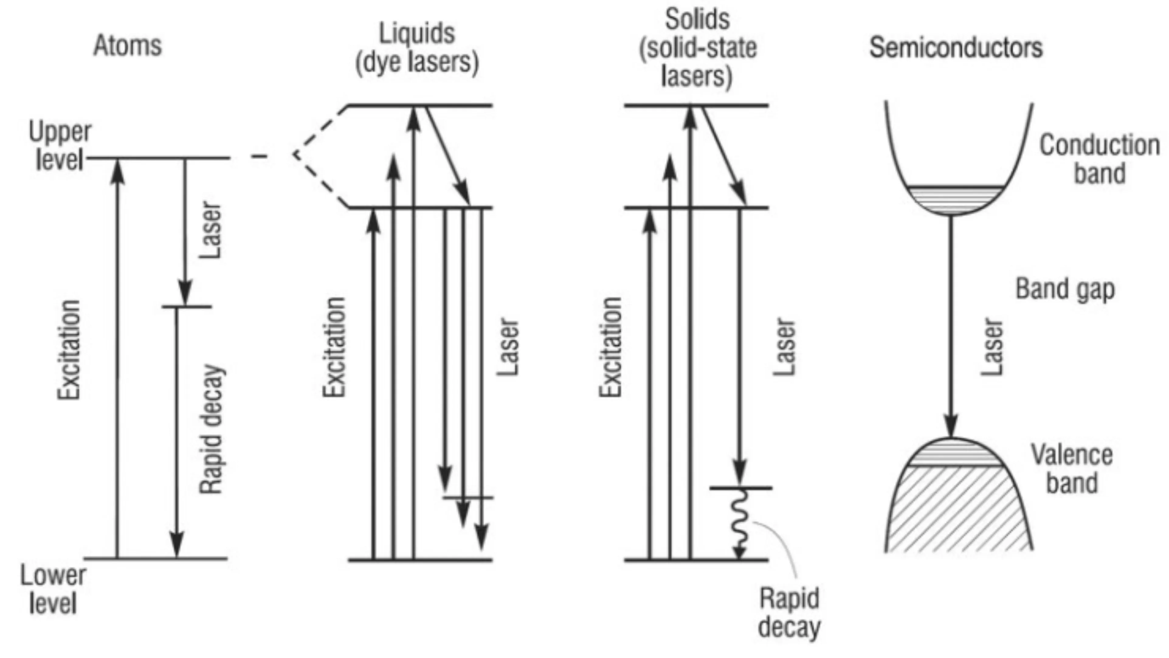
A variety of pumping schemes are used to deliver energy to the gain medium. Some examples include:

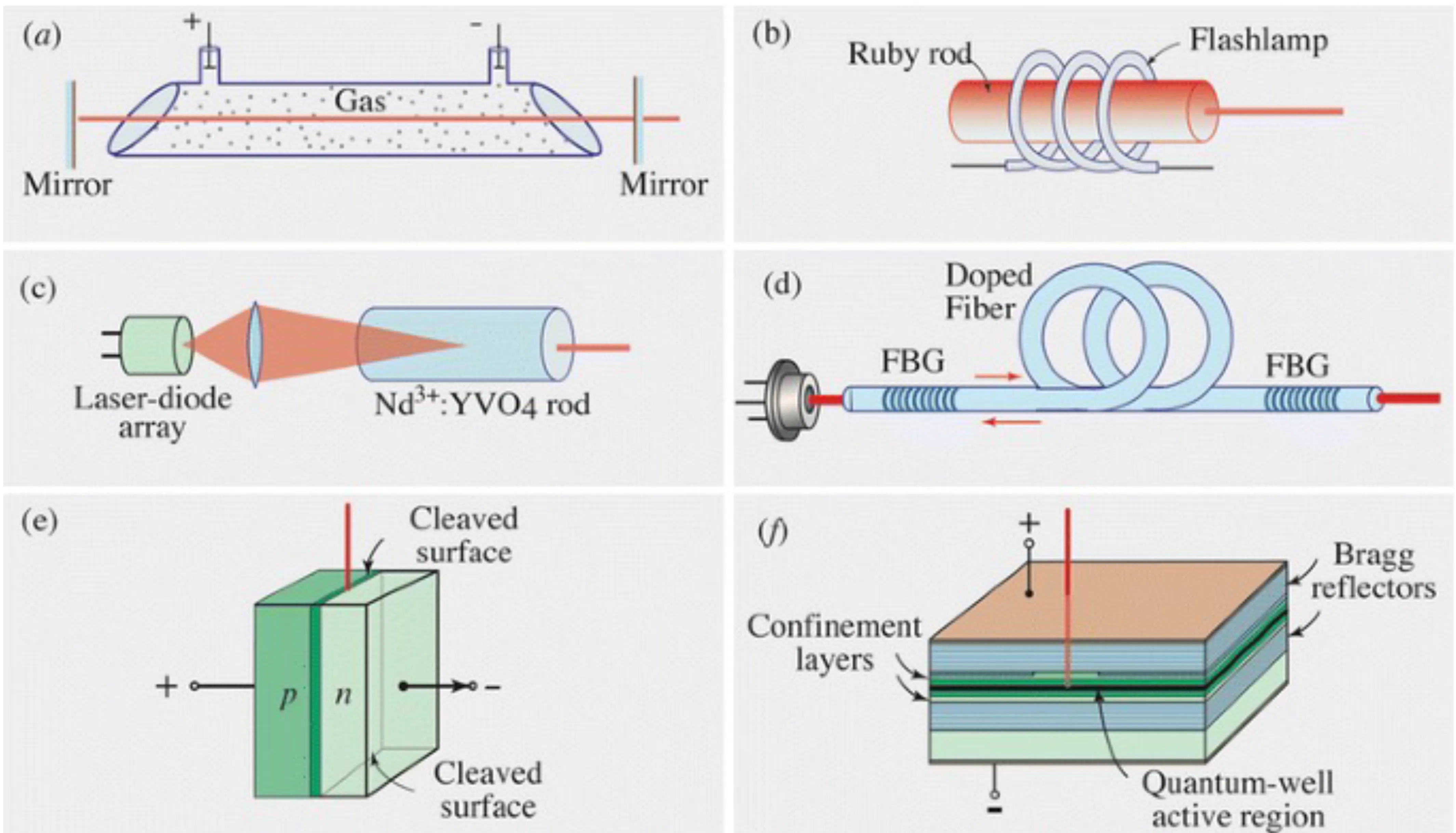
• (a) Gas laser pumped by direct current (DC) electrical discharge.
• (b) Solid-state laser pumped by a flashlamp.
• (c) ${\text{Nd:YVO}}_4$ solid-state laser optically pumped by a laser diode array.
• (d) Fibre laser (such as erbium-doped silica fibre) with fibre Bragg grating reflectors, pumped with a laser diode.
• (e) Laser diode (a forward-biased p-n junction) with cleaved facets acting as mirrors, pumped by electrical current injection.
• (f) Quantum-well semiconductor laser, pumped electrically.

8.4 Laser Rate Equations

We will treat an ideal four-level system in more detail. Assume an ideal system where ${\tau }_{32}\to 0$ (atoms pumped to $|3⟩$ immediately transfer to $|2⟩$) and ${\tau }_{10}\to 0$ (atoms arriving in $|1⟩$ immediately decay to $|0⟩$, so $N_1\approx 0$). The lasing transition is $|2⟩\to |1⟩$.

Consider a single lasing mode within the cavity, and assume a homogeneously broadened gain medium. Let $n$ be the number of photons in the lasing mode and $N_2$ be the population density of the upper laser level (we can denote $N_2\equiv N_{\text{inv}}$ as the inversion density, since $N_1\approx 0$). Two coupled rate equations can describe the system:

where:

• $K$ is a coupling constant proportional to the stimulated emission cross-section and mode volume ($K\sim B_{21}$).
• $K{N}_{\text{inv}}$ is the rate of spontaneous emission into the lasing mode (the "+1" in $K(n+1)N_{\text{inv}}$ from some texts is written as $K{N}_{\text{inv}}$ here, as spontaneous emission into the mode).
• $Kn{N}_{\text{inv}}$ is the rate of stimulated emission into the lasing mode.
• ${\gamma }_c$ is the cavity photon decay rate (loss rate from cavity, ${\gamma }_c=1/{\tau }_{\text{photon}}$, where ${\tau }_{\text{photon}}$ is photon lifetime).
• $R_p$ is the pumping rate into the upper laser level $N_2$.
• ${\gamma }_L$ is the total decay rate of the upper laser level $N_2$ due to all processes other than stimulated emission into the lasing mode (primarily spontaneous emission, ${\gamma }_L\approx 1/{\tau }_{21}$).

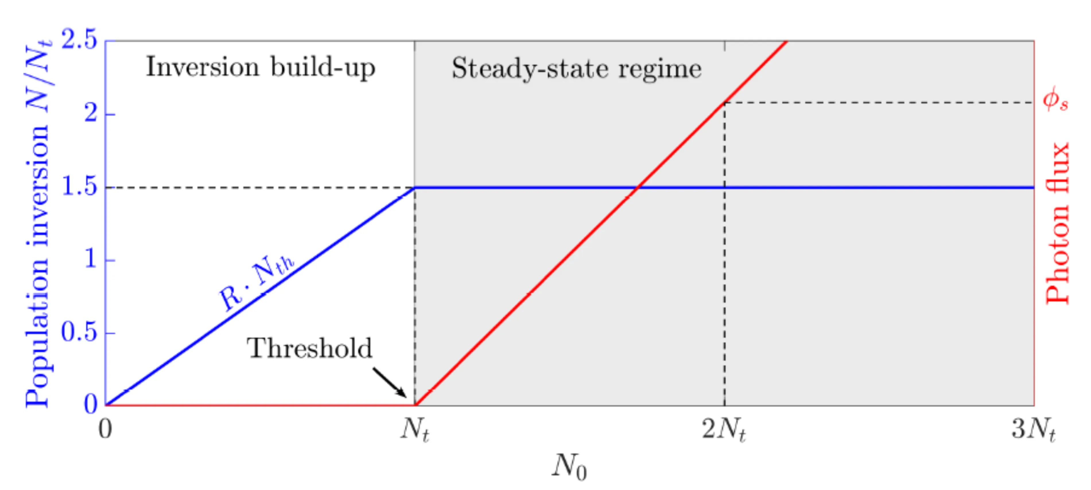
In stationary solutions ($dn/dt=0,d{N}_{\text{inv}}/dt=0$):
From the first equation (for $n>0$): $K(n_s+1)N_s={\gamma }_c{n}_s⟹(K{N}_s-{\gamma }_c)n_s=-K{N}_s$.
This implies $K{N}_s={\gamma }_c$ for steady-state lasing (gain equals loss), assuming $n_s\gg 1$ so the spontaneous term $K{N}_s$ is small compared to $K{n}_s{N}_s$.
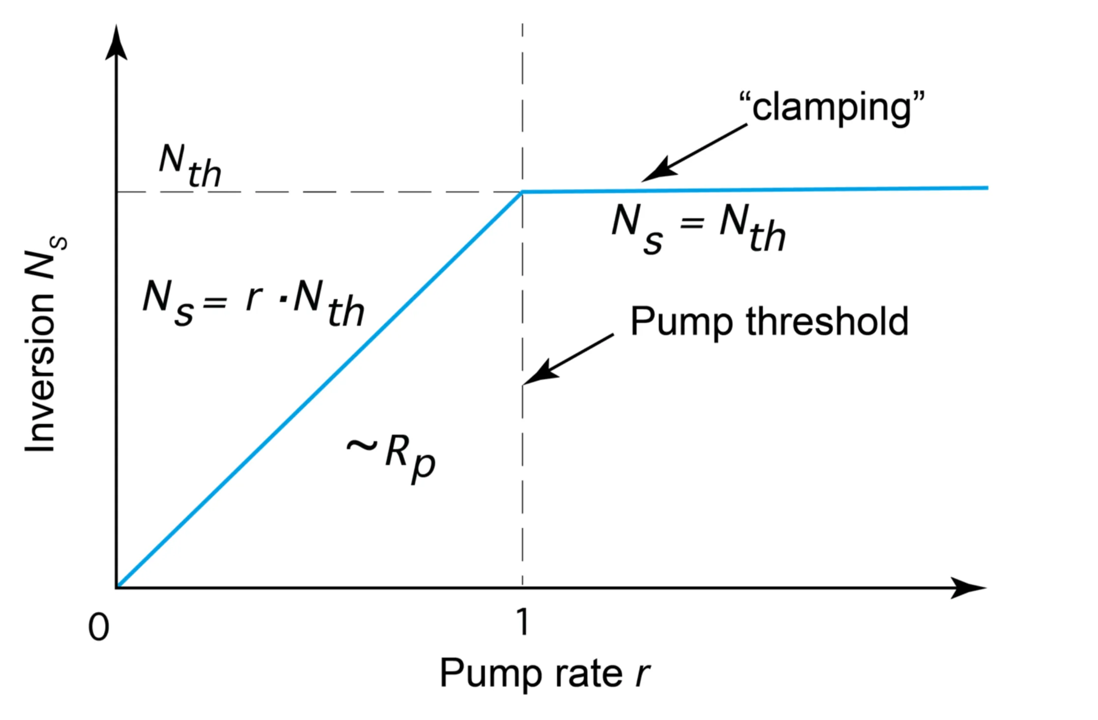
This defines the threshold inversion density:

Above threshold, the inversion clamps at $N_s\approx N_{\text{th}}$.
From the second equation, $R_p=K{n}_s{N}_s+{\gamma }_L{N}_s$. Substituting $N_s\approx N_{\text{th}}$ for $r>1$:

The threshold pumping rate $R_{p,th}$ is when $n_s\approx 0$, so $R_{p,th}\approx {\gamma }_L{N}_{\text{th}}=\frac{{\gamma }_L{\gamma }_c}{K}$.
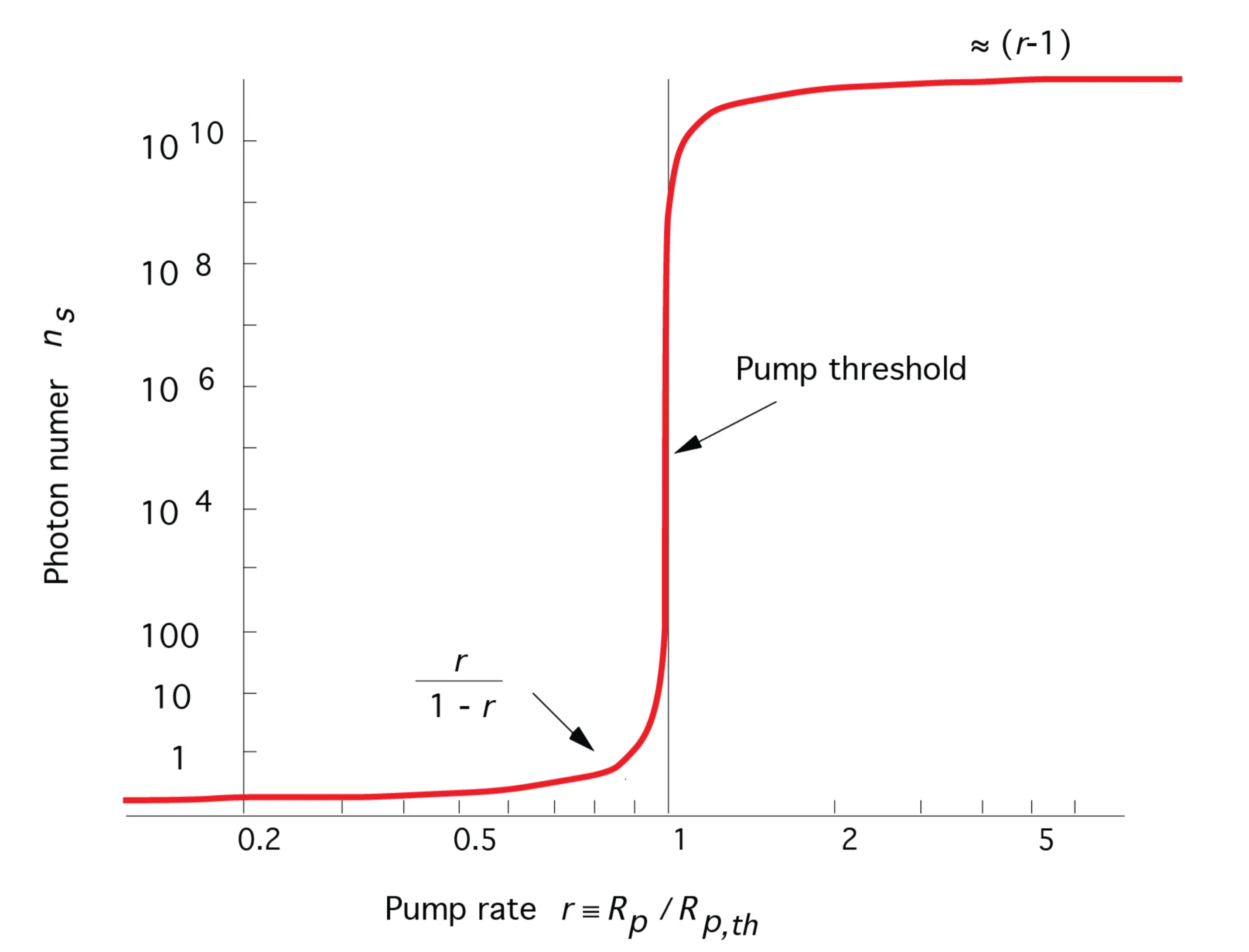
Let $r=R_p/R_{p,th}$ be the normalised pumping rate.
Then $n_s\approx \frac{{\gamma }_L}{K}(r-1)$.

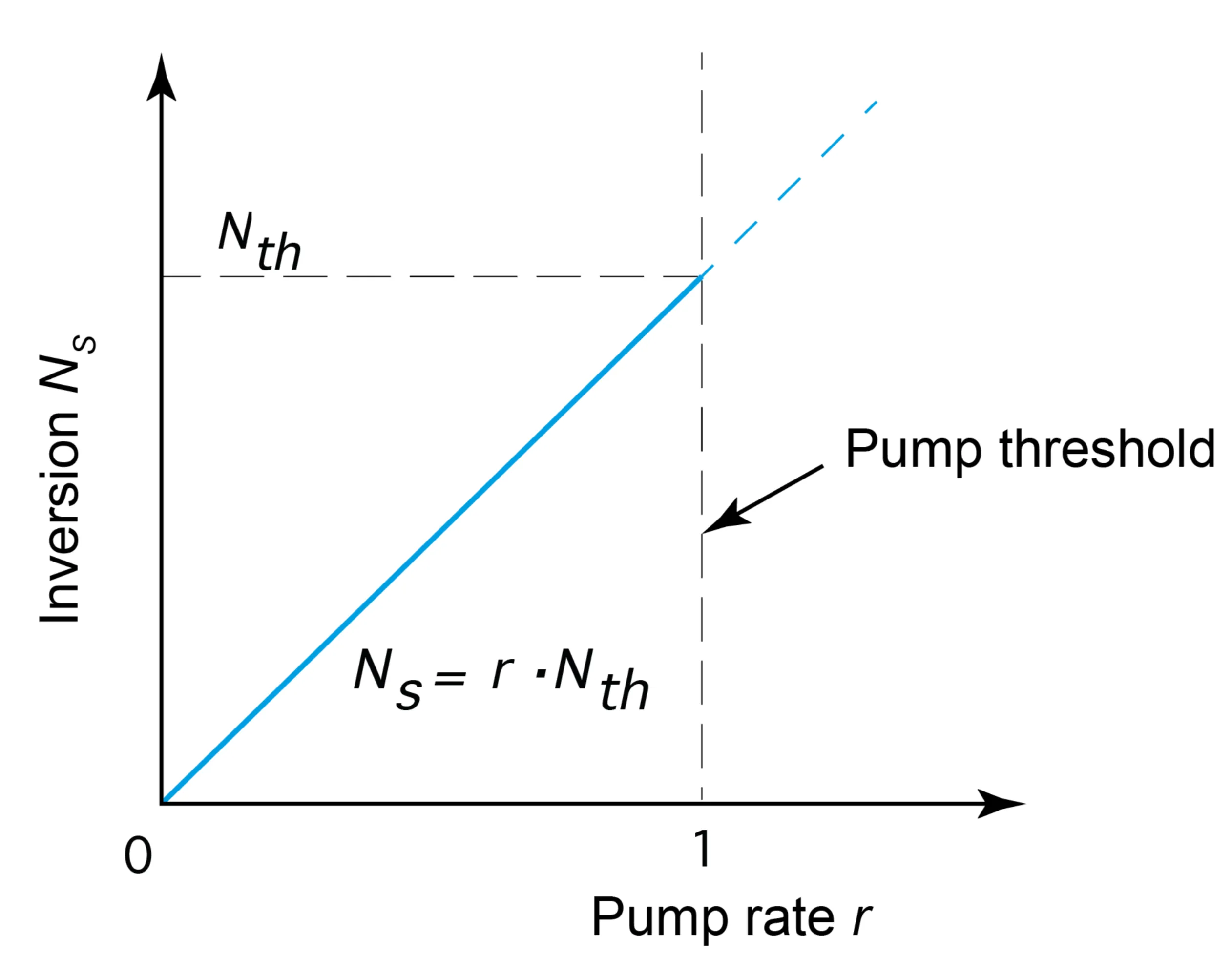
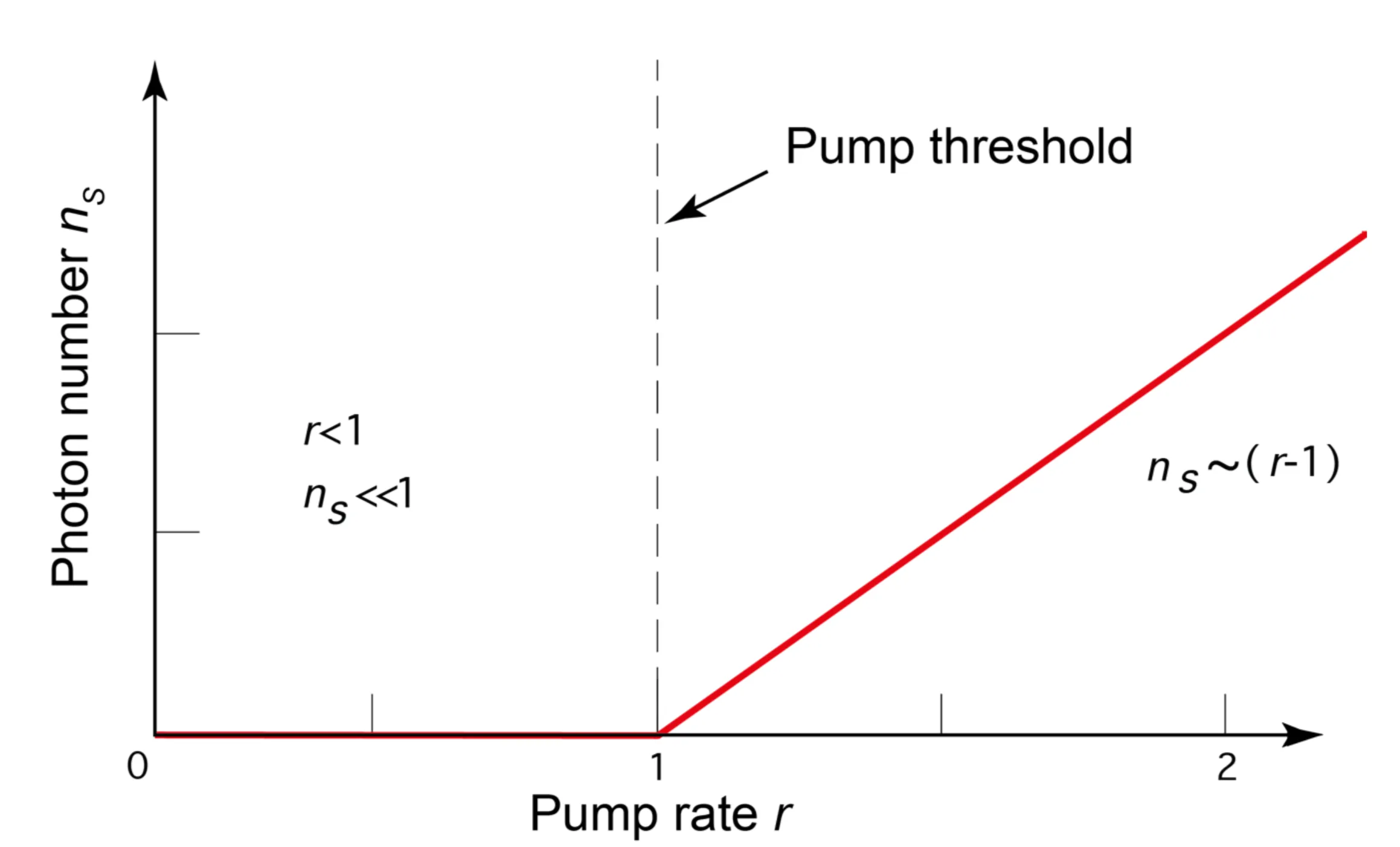
• Above threshold ($r>1$):$$N_s\approx N_{\text{th}}=\frac{{\gamma }_c}{K}$$$$n_s\approx \frac{{\gamma }_L}{K}(r-1)$$The inversion is clamped to its threshold value. Every additionally pumped atom primarily contributes to stimulated emission, increasing the coherent photon number $n_s$.
• Below threshold ($r<1$):
  Stimulated emission is negligible ($n_s\approx 0$). $d{N}_{\text{inv}}/dt\approx R_p-{\gamma }_L{N}_s=0⟹N_s\approx R_p/{\gamma }_L=r{R}_{p,th}/{\gamma }_L=r(N_{\text{th}}/{\tau }_L){\tau }_L=r{N}_{\text{th}}$.
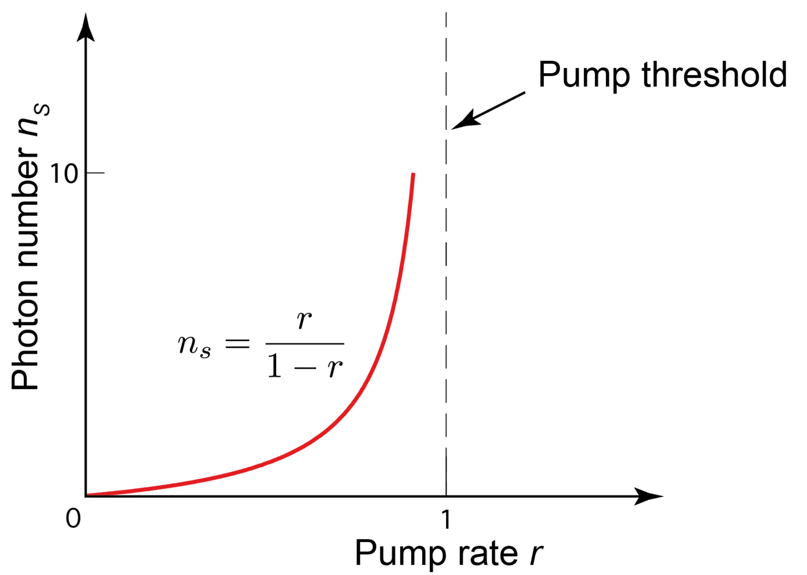
  The photon number $n_s$ is very small, dominated by spontaneous emission into the mode: $n_s\approx K{N}_s/{\gamma }_c=K(r{N}_{\text{th}})/{\gamma }_c=r$.

The output power is proportional to $n_s$. Well above threshold ($r\gg 1$), the photon number $n_s$ (and thus output power) is approximately linearly proportional to the pump rate $R_p$.

The exact solutions show a smooth transition around the threshold:

8.5 Experimental Parameters of Lasers

In practice, inversion and photon number are not always the most directly accessible experimental quantities. Gain, loss, and output power (related to photon flux) are often more useful.
The gain coefficient is $\gamma (\nu )=N_{\text{inv}}{\sigma }_{em}(\nu )$, where $N_{\text{inv}}=N_2-(g_2/g_1)N_1$.
The small-signal gain coefficient (unsaturated gain) is ${\gamma }_0(\nu )=N_{0,\text{inv}}{\sigma }_{em}(\nu )$, where $N_{0,\text{inv}}$ is the inversion achieved by pumping in the absence of cavity photons ($n\approx 0$).
Gain clamping above threshold means $N_s\approx N_{\text{th}}$, so the actual gain coefficient in steady-state lasing clamps at the threshold value required to overcome losses.
The resonator losses $l$ per round trip consist of unwanted losses (absorption, scattering, diffraction) and output coupling losses $T_{oc}$ (transmission through the output mirror). If $R_1,R_2$ are mirror power reflectivities, $l=(1-R_1{R}_2)+\text{internal losses}$.
After one resonator round trip of length $L_{\text{RT}}=2L$ (for a linear cavity of length $L$), the intensity reduces by a factor $e^{-l}$. The cavity photon decay rate ${\gamma }_c$ is related to losses by ${\gamma }_c=lc/(n{L}_{\text{RT}})=l/T_R$, where $T_R=n{L}_{\text{RT}}/c$ is the round-trip time.
The total round trip gain (power) is $G(\nu )=e^{2\gamma (\nu )L_g}$ (where $L_g$ is length of gain medium).
The net gain per round trip $G_{\text{net}}=G(\nu )e^{-l}$. For steady-state lasing, $G_{\text{net}}=1$, so $2\gamma (\nu )L_g=l$. The gain must equal the losses.
Thus, $\gamma (\nu )=l/(2L_g)$. The gain coefficient clamps to this value.
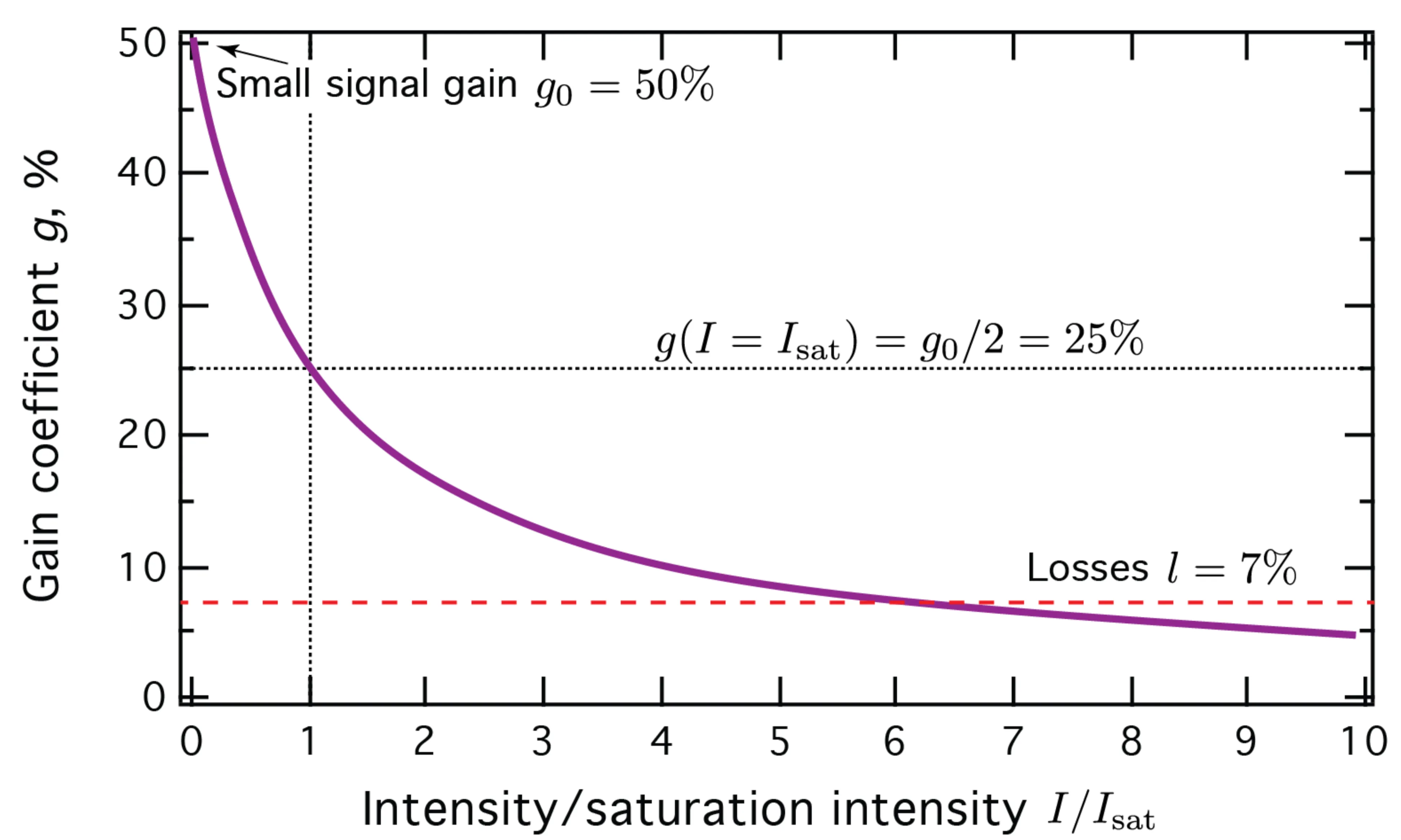
The gain coefficient saturates with increasing intra-cavity intensity $I$ (or photon flux $\varphi$) as:

where $I_{\text{sat}}$ and ${\varphi }_{\text{sat}}$ are the saturation intensity and saturation photon flux, respectively.
$I_{\text{sat}}=\frac{h\nu }{{\sigma }_{em}{\tau }_{21}}$ where ${\tau }_{21}$ is the upper laser level lifetime (including all decay channels). The saturation fluence is $F_{\text{sat}}=I_{\text{sat}}{\tau }_{21}=h\nu /{\sigma }_{em}$.
Both saturation intensity and fluence are material and transition-specific properties.

Gain clamping:

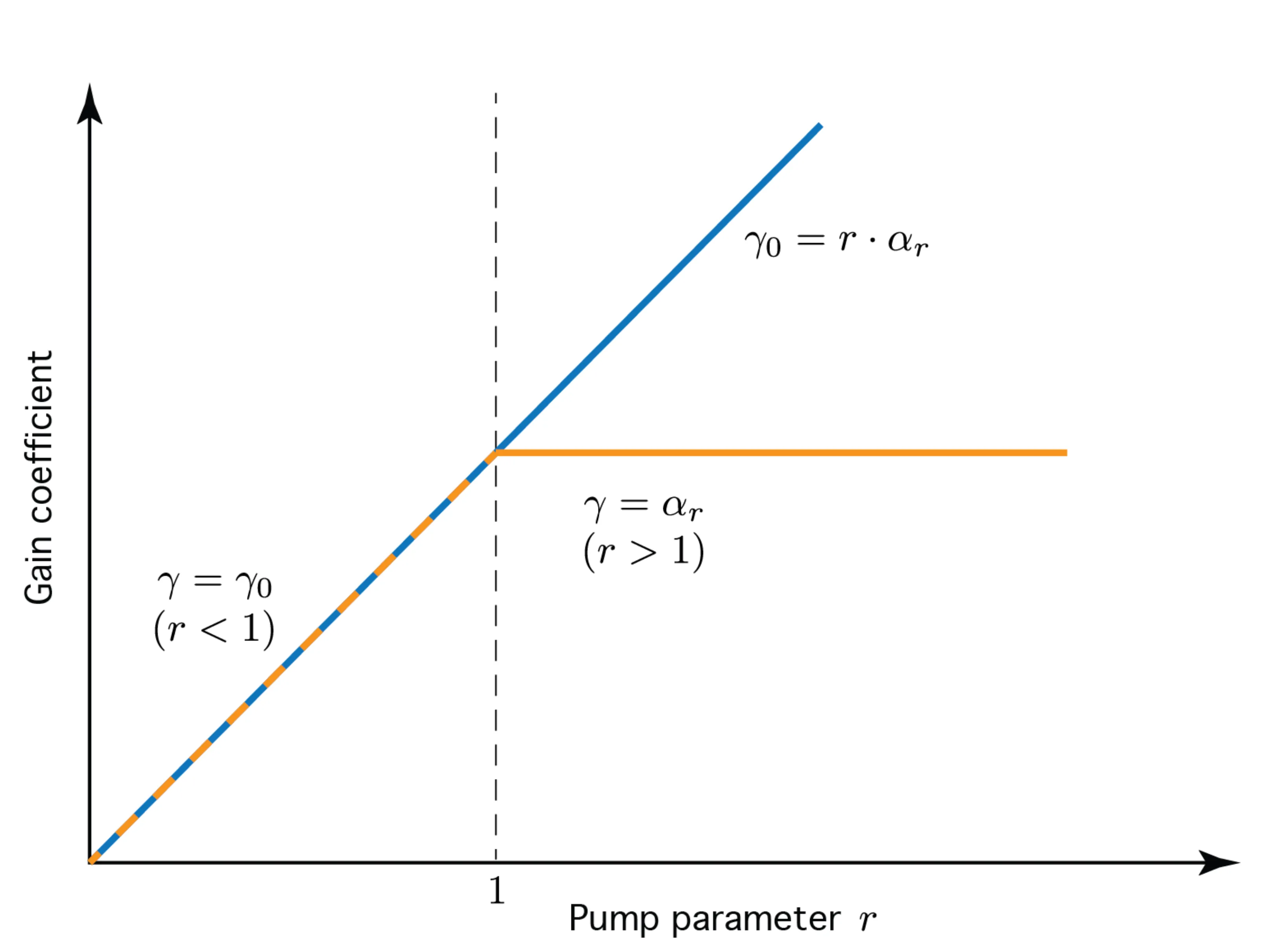
The small-signal gain ${\gamma }_0$ increases with pump power. The actual gain $\gamma$ clamps at the threshold value (gain = losses) once lasing starts. At saturation intensity $I=I_{sat}$, the gain is reduced to ${\gamma }_0/2$.

Figure shows gain $g=\gamma L_g$.

8.6 Initial Laser Dynamics

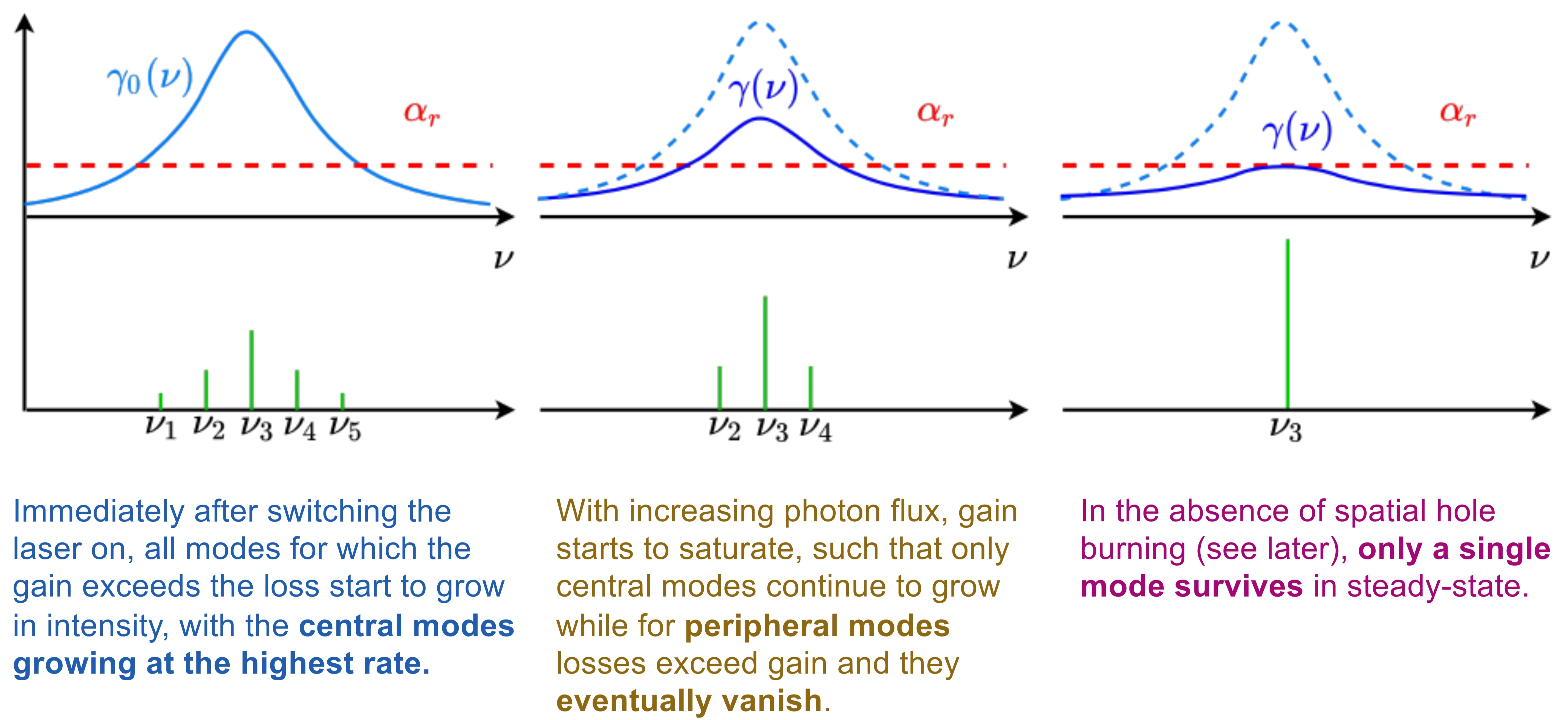
Initially, when pumping starts, the photon flux in the cavity is negligible (originating from spontaneous emission). The population inversion $N_{\text{inv}}$ builds up towards its small-signal value $N_0$. Eventually, by chance, a spontaneously emitted photon will be emitted into a cavity mode that has net gain ($2{\gamma }_0{L}_g>l$). This photon initiates stimulated emission. As the photon flux builds up through many round trips of amplification, it starts to deplete the population inversion (gain saturation). The gain is reduced until it exactly balances the losses. The photon flux then asymptotically reaches its steady-state value.

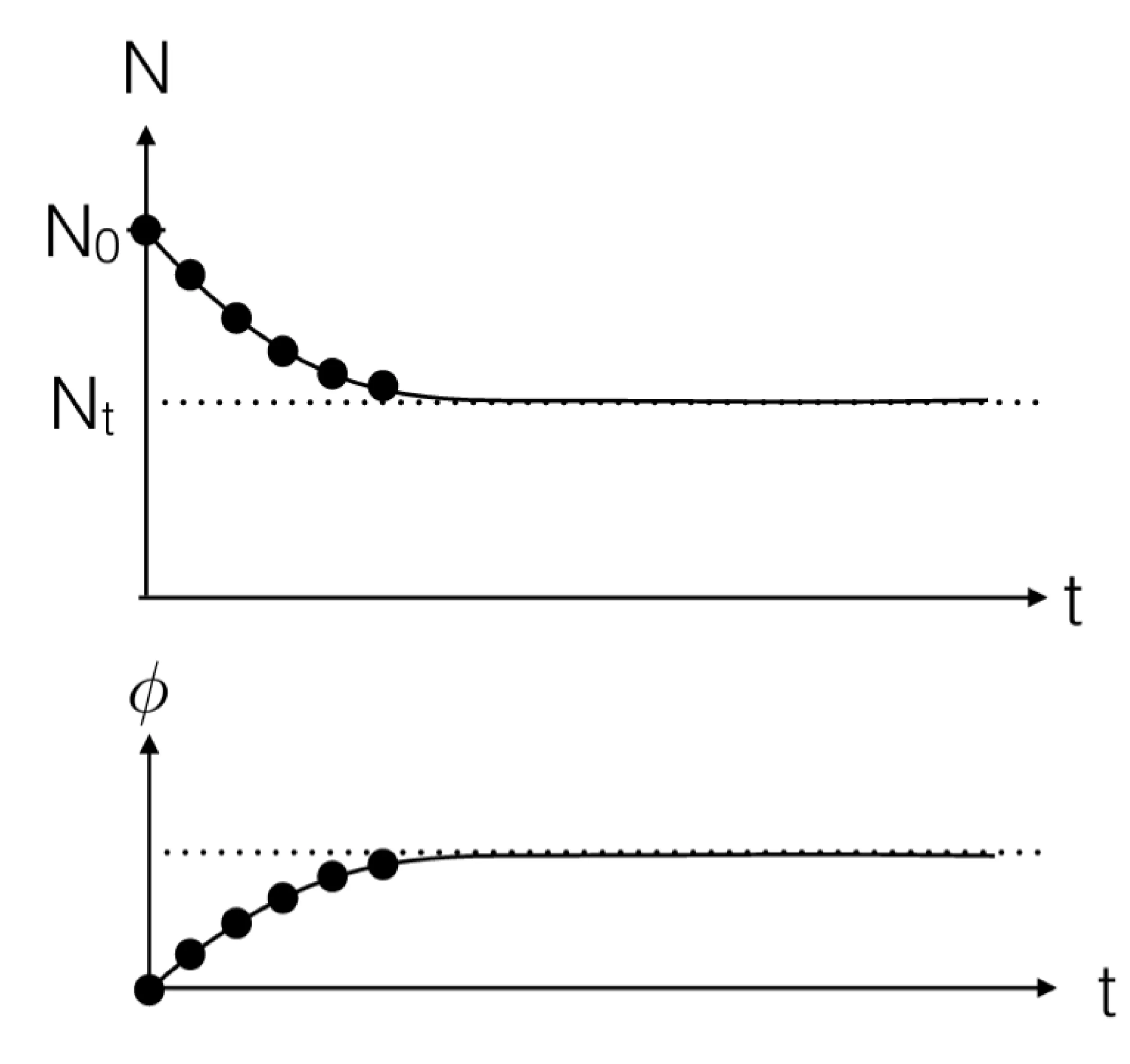
Initially, there is primarily incoherent spontaneous emission. As lasing threshold is reached and surpassed, coherent stimulated emission into one or a few cavity modes dominates. The total spontaneous emission into all $4\pi$ steradians may still occur, but the output beam consists mainly of coherent light.

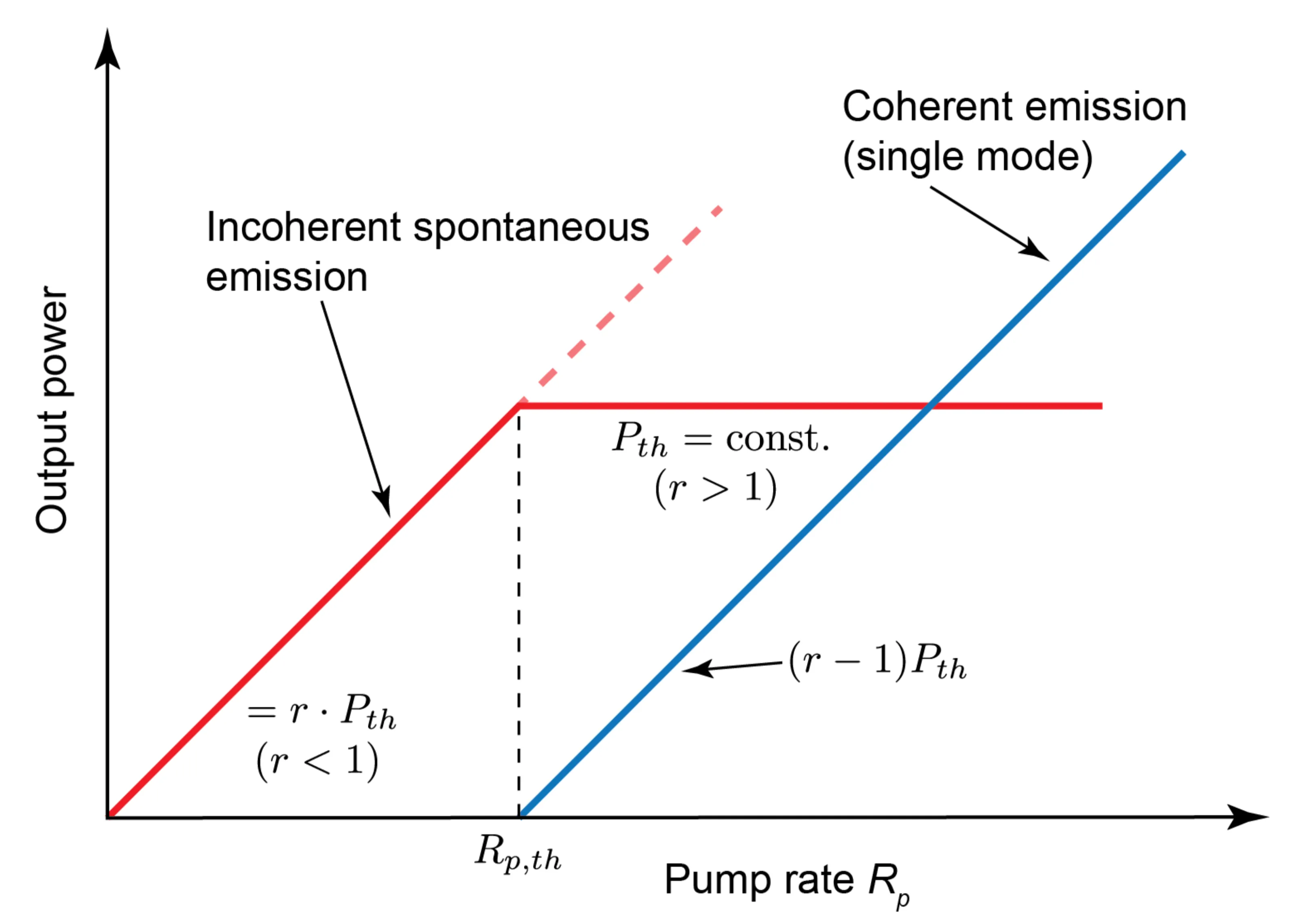
Above threshold, pumping harder primarily increases the flux of coherent photons, while the population inversion (and thus gain) remains clamped at the threshold value $N_{\text{th}}$.

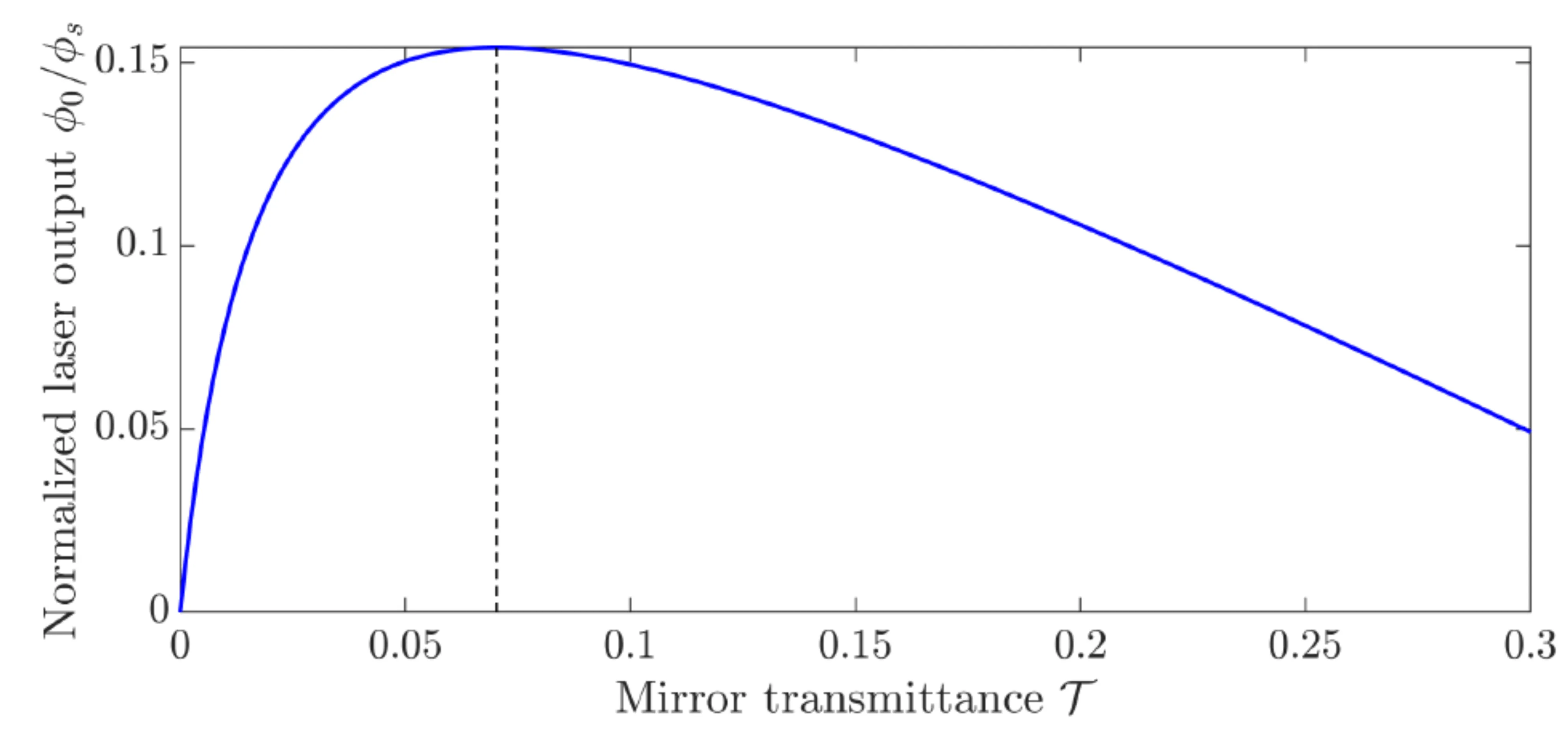
To optimise the laser output power $P_{out}\sim {\varphi }_{out}$, consider one mirror perfectly reflecting and the other having a power transmittance $\mathcal{T}$ (output coupler). The output photon flux ${\varphi }_{out}$ is related to the intracavity flux ${\varphi }_{intra}$ by ${\varphi }_{out}={\varphi }_{intra}\mathcal{T}/(\text{round trip factor})$. It can be shown that an optimal transmittance ${\mathcal{T}}_{opt}$ exists that maximises output power for given laser parameters.

Another useful form for the threshold inversion density is:

This shows that it is more difficult to reach threshold (higher $N_{th}$) for shorter wavelengths (due to ${\lambda }_0^2$ in denominator) and for frequencies away from the peak of the gain lineshape $g(\nu )$. This is one reason why building, for instance, ultraviolet or X-ray lasers is challenging.

8.7 Mode Selection

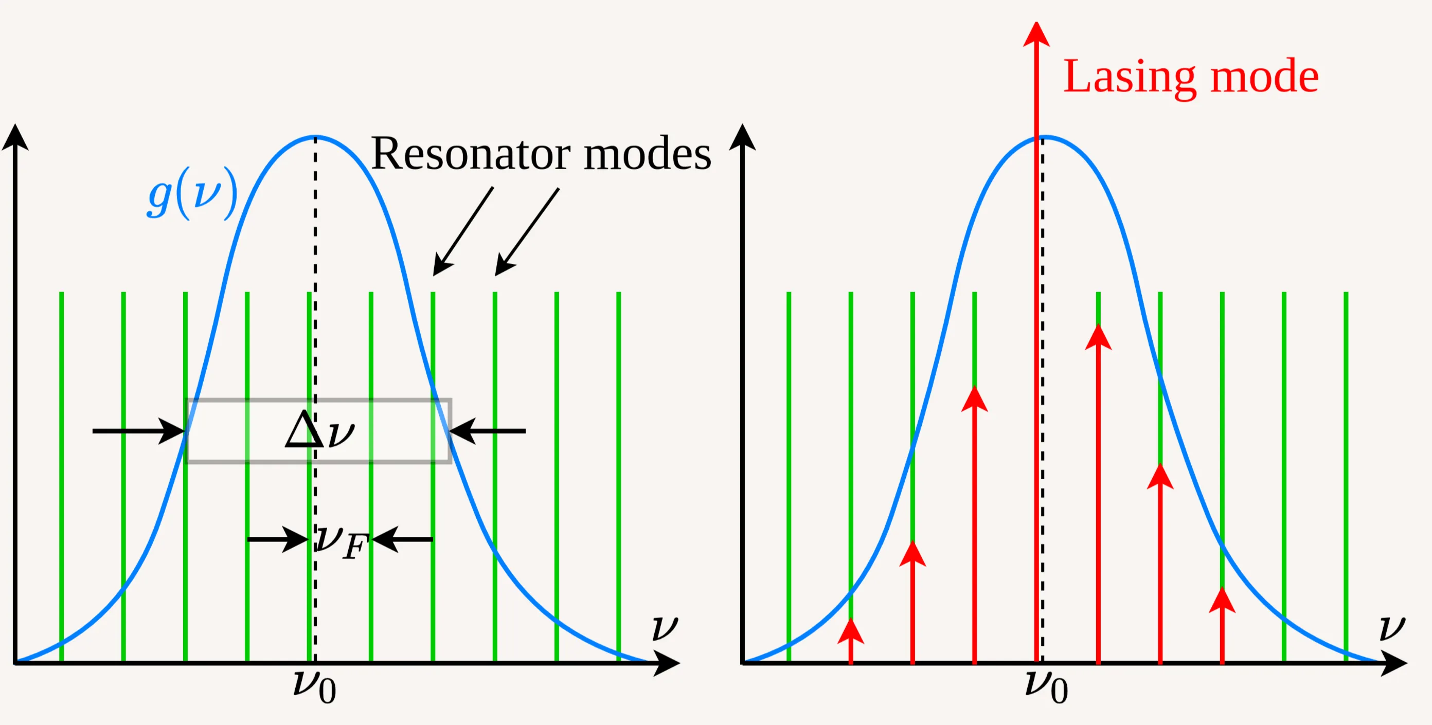
So far, we have assumed that the energy emitted by an atomic transition is quantised, ideally leading to emitted light at a single frequency ${\nu }_0=(E_2-E_1)/h$. However, we have also seen that in reality, broadening effects give the gain spectrum a finite width $g(\nu )$. Additionally, an optical cavity supports a discrete set of resonant modes (longitudinal and transverse). Longitudinal modes are narrowly peaked in frequency, spaced by the Free Spectral Range (FSR). These cavity resonances are typically much narrower than the gain bandwidth $g(\nu )$.
Lasing will occur preferentially for those cavity modes that fall within the gain bandwidth $g(\nu )$ and for which the gain exceeds the losses. The cavity modes gain energy over many round trips through amplification by stimulated emission. In a multi-mode laser, several longitudinal modes may lase simultaneously. In many single-mode lasers, the cavity mode closest to the peak of the gain lineshape will experience the highest net gain and will dominate over other modes. As it builds up intensity, it saturates the gain medium, potentially suppressing other modes below their threshold.

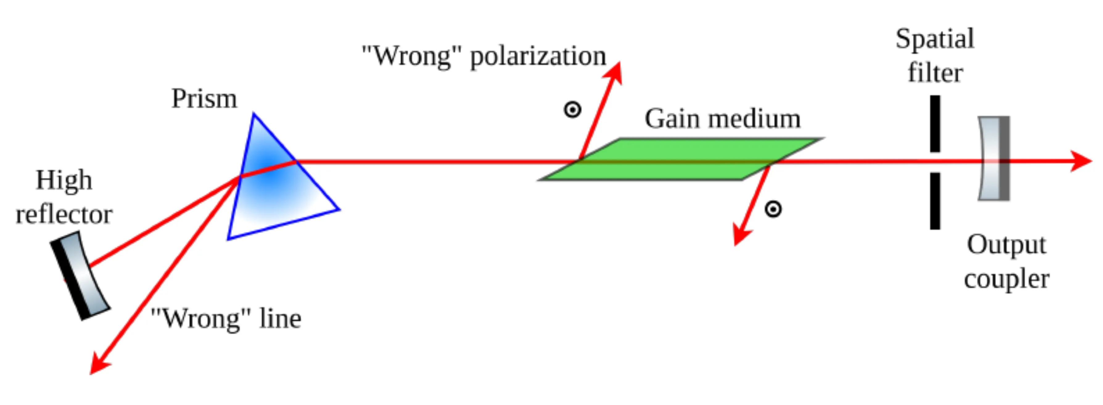
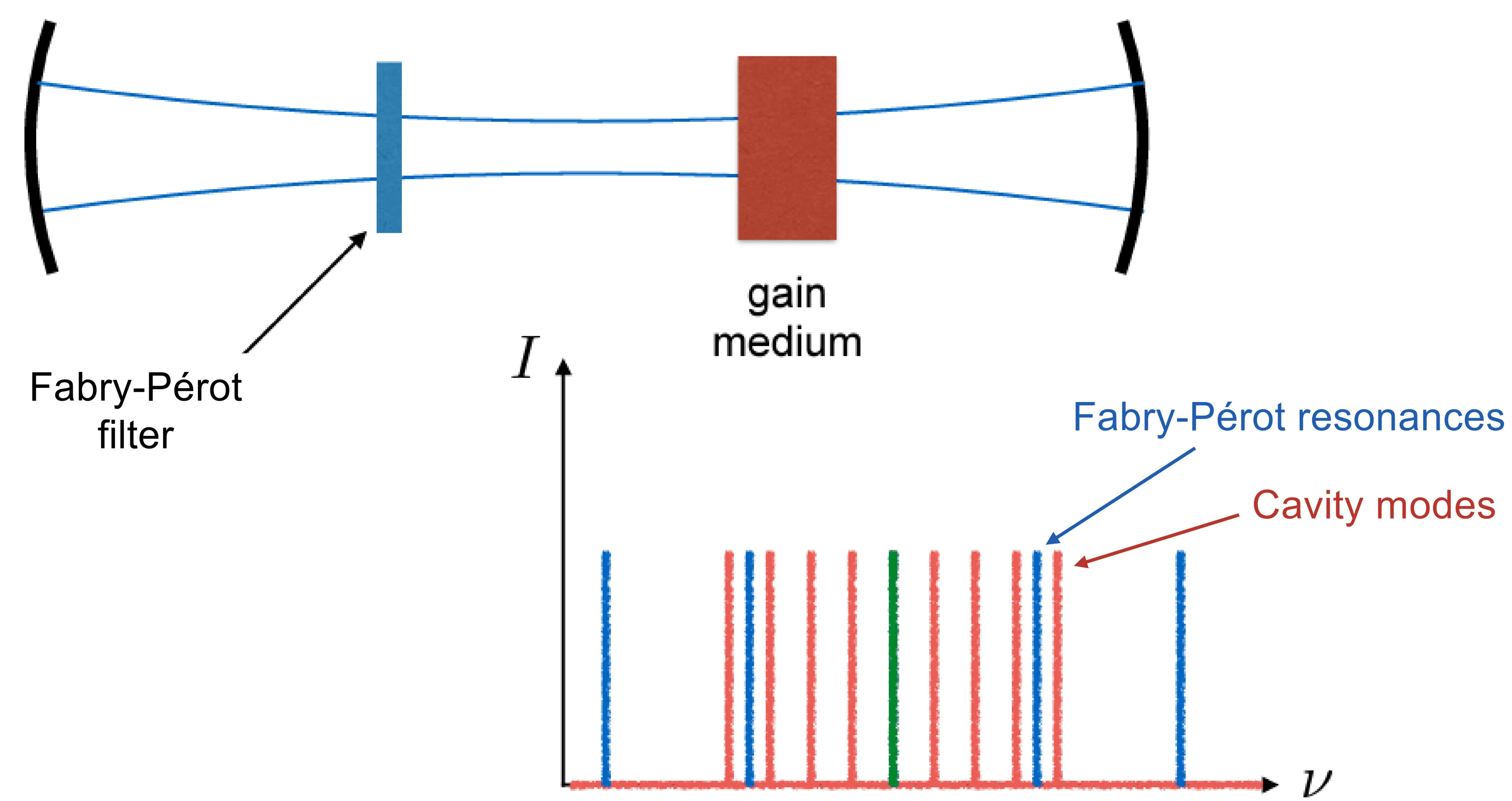
For some applications, single-longitudinal-mode operation is required. This can be achieved by introducing spectrally selective loss elements into the cavity (such as etalons or birefringent filters) to ensure only one desired mode remains above threshold. The following figures show some methods for longitudinal mode selection:

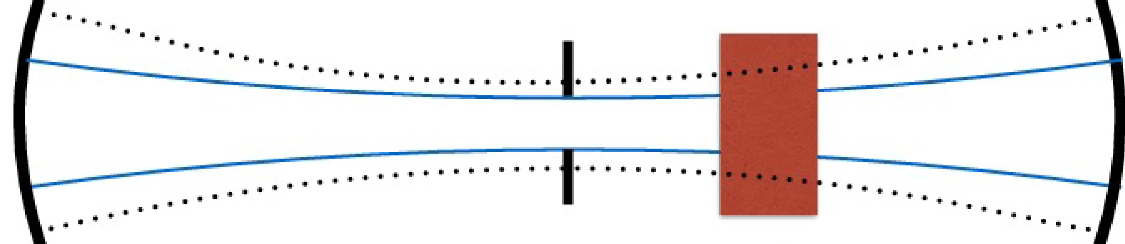
Selection of a single transverse mode (typically the fundamental $TE{M}_{00}$ Gaussian mode) is also crucial for good beam quality. Transverse modes depend on the resonator geometry and can experience different diffraction losses, for instance, due to finite mirror sizes or intracavity apertures. By carefully designing the resonator and potentially including an aperture, higher-order transverse modes (which are typically larger in spatial extent) can be made to experience higher losses, thus ensuring fundamental mode operation.

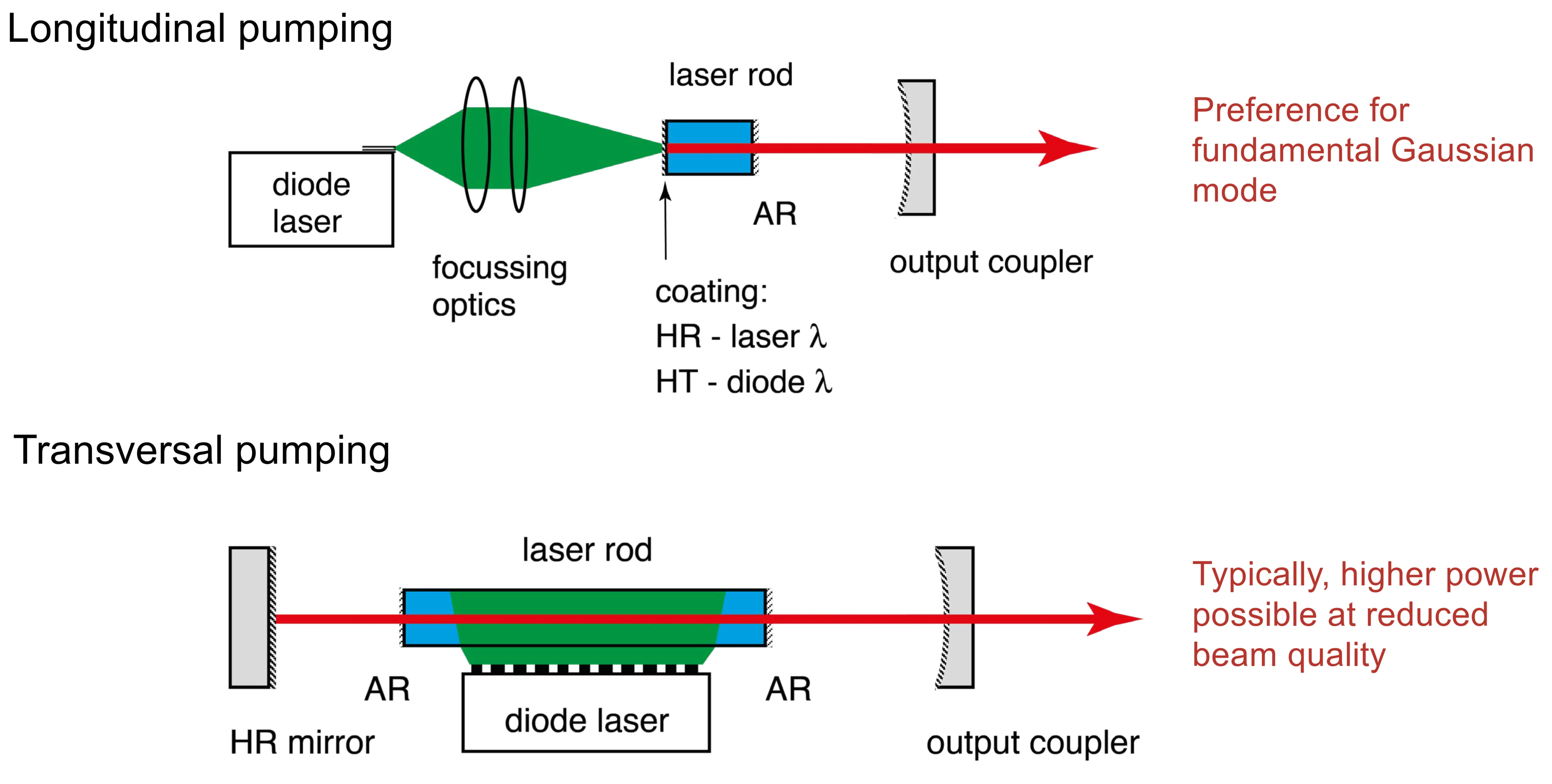
Mode selection also depends on the type of pumping scheme and how well the pumped volume in the gain medium overlaps with the desired lasing mode volume:

8.8 Hole Burning

There are two main types of hole burning relevant to lasers:

• Spatial hole burning: This occurs in linear laser resonators where a standing wave intensity pattern is formed by the counter-propagating waves. Gain saturation is strongest at the antinodes of this standing wave and weakest at the nodes. This means that near the standing wave minima, the gain is not effectively saturated by the lasing mode. Consequently, other longitudinal modes, whose standing wave patterns might have antinodes where the primary mode has nodes, can reach threshold and lase. This leads to multi-mode operation. Ring laser cavities, where light propagates in one direction, avoid the formation of strong standing waves and thus mitigate spatial hole burning.
• Spectral hole burning: This occurs predominantly in inhomogeneously broadened gain media. When a particular longitudinal mode starts lasing at frequency ${\nu }_L$, it primarily interacts with and saturates only those atoms (or molecules) whose individual resonance frequencies are close to ${\nu }_L$. Once these atoms are saturated, they no longer contribute significantly to the gain at ${\nu }_L$. This effectively "burns a hole" in the gain spectrum at that frequency, reducing the gain for that specific mode. Other modes at different frequencies, interacting with different sub-ensembles of atoms, might still be above threshold.

8.9 Pulsed Lasers - Overview

Previously, the discussion largely focused on continuous wave (CW) and single-mode lasers, which (ideally) have a constant intensity output as a function of time. Very often, however, pulsed laser operation is desired, as pulsed lasers are crucial for a wide range of applications. The average power of a laser is typically limited by thermal effects in the gain medium and pump source capabilities. A laser emitting short pulses essentially concentrates its energy into very brief intervals of light, which in turn leads to very high peak power and peak intensity, even if the average power is moderate. High peak power enables various nonlinear optical applications important for industrial processes and scientific research. Furthermore, short pulses allow for high time-resolution in measurements of dynamical processes, such as molecular vibrations or even electronic wavepacket motion. These measurements and techniques form the core of Ultrafast Laser Physics. The following is an overview of common methods to produce laser pulses.

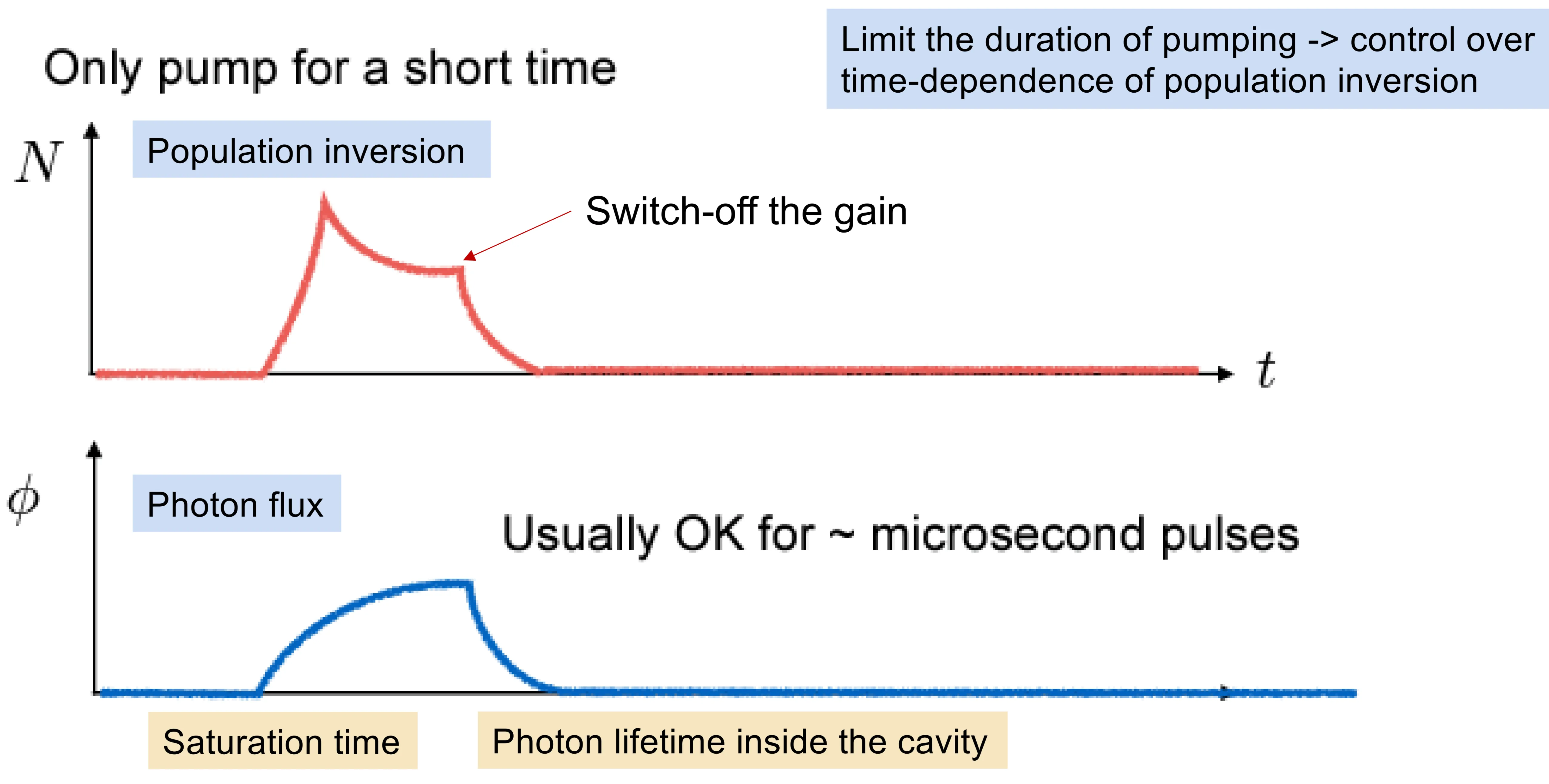
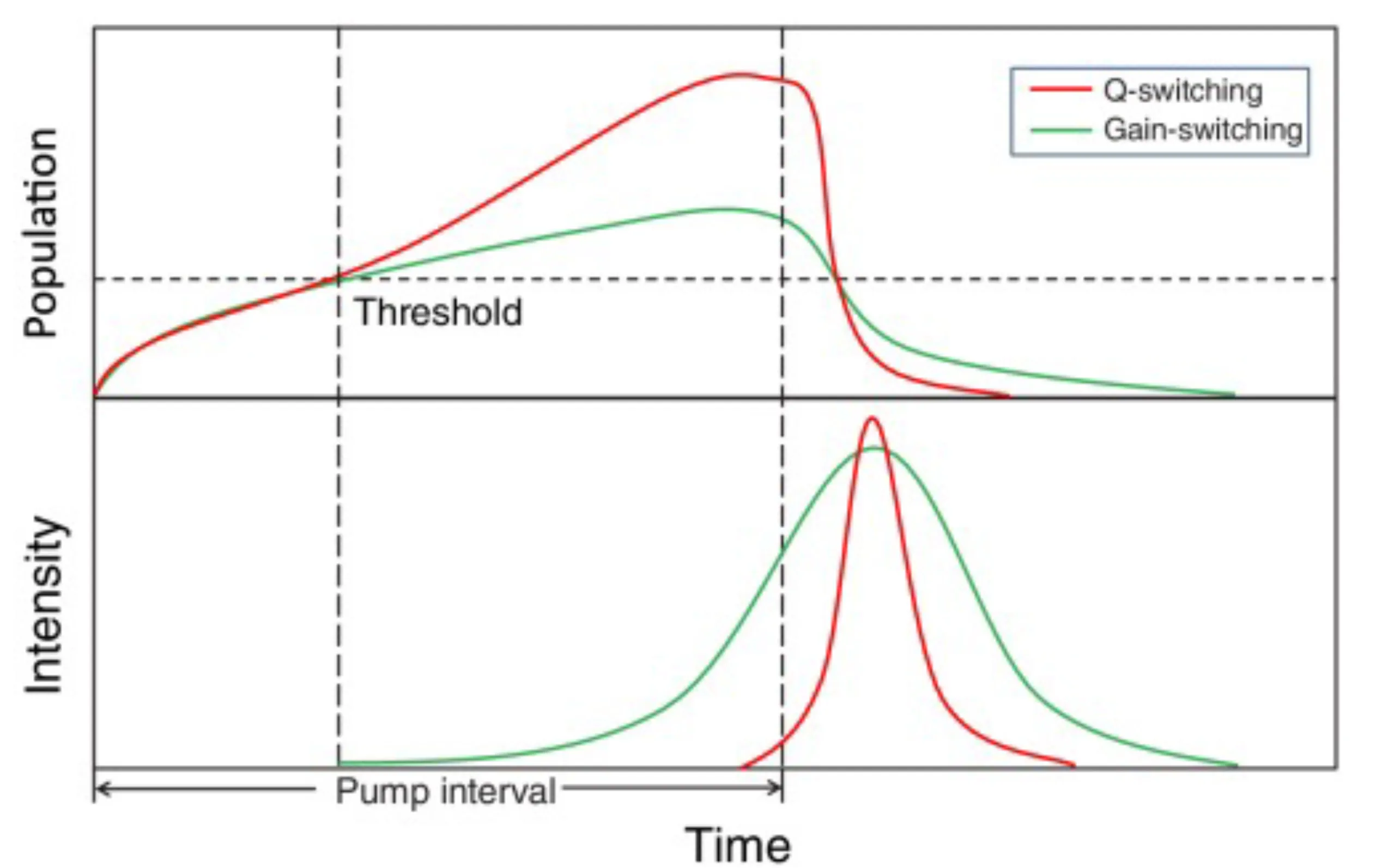
• Gain Switching: This is perhaps the simplest technique to produce pulses of light. The pump source is rapidly turned on and off, effectively switching the gain above and below the threshold. The duration of the pulses achievable with this method is limited by several timescales, including the initial build-up time of photons in the cavity and the decay time after the gain is switched off, both of which depend on the gain medium and cavity properties. The speed of switching the pump (and thus the gain) also limits the pulse duration. This method is typically suitable for generating relatively long pulses, with durations of several microseconds or longer.
  
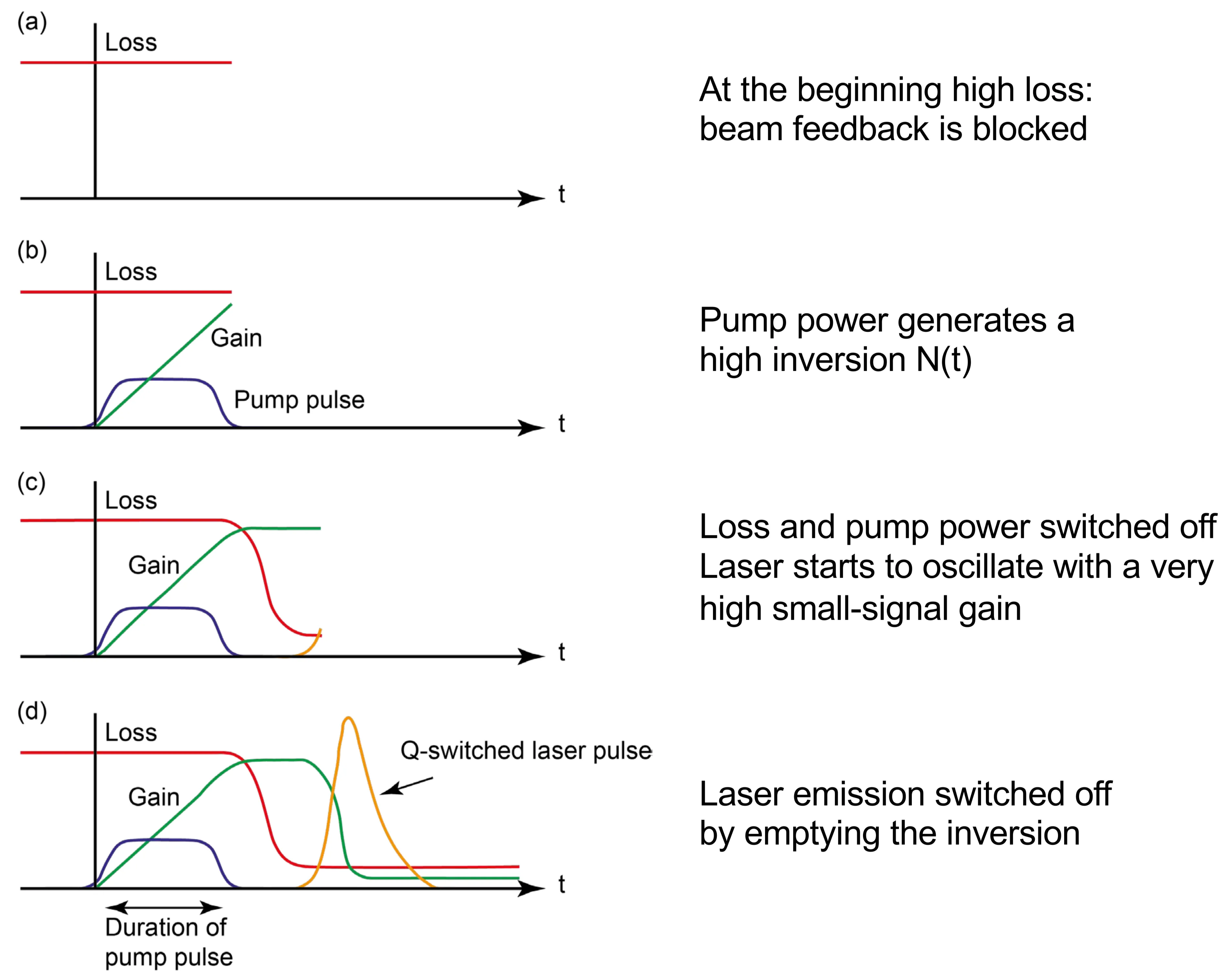
• Q-Switching: This method involves modulating the quality factor (Q-factor) of the laser cavity, which is inversely related to the cavity losses. Lasing requires gain to exceed losses. The idea is to initially keep the cavity losses very high (low Q), suppressing lasing, which allows the pump to build up a very large population inversion in the gain medium, far above the normal threshold level. At a chosen moment, the losses are suddenly reduced (Q is switched to a high value). With the gain now significantly exceeding the (lowered) losses, stimulated emission rapidly depopulates the inversion, releasing the stored energy as a short, intense pulse of light. This Q-switching can be achieved using active modulators (such as electro-optic or acousto-optic switches) or passive saturable absorbers. Compared to gain switching, the population inversion is already established at a high level before the pulse emits, allowing for shorter pulse durations and much higher peak powers. It is the method of choice for achieving pulses with large pulse energy (millijoules to joules). The duration is typically limited to nanoseconds.
  
  
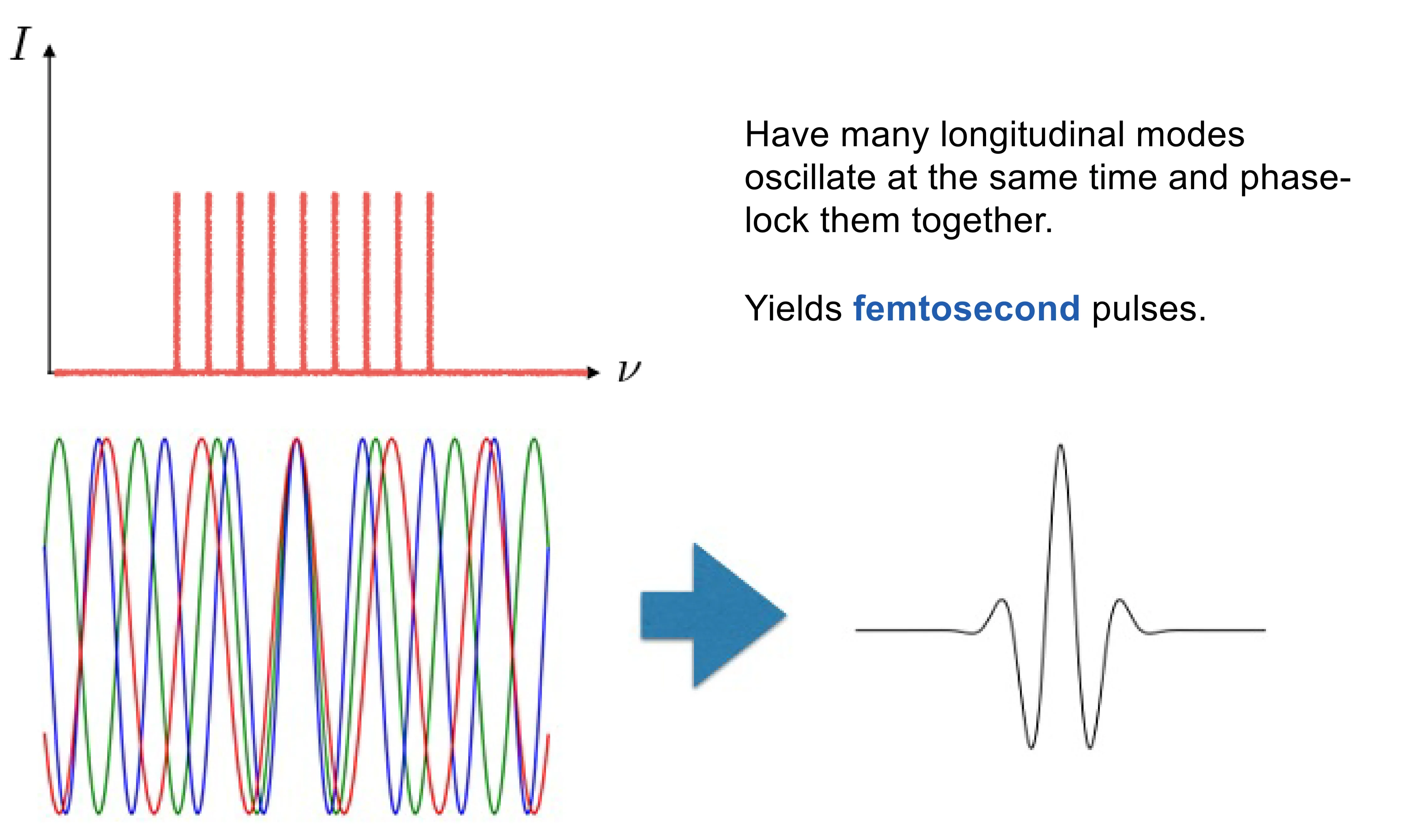
• Mode-locking (active/passive): This technique allows the generation of the shortest pulses directly from a laser cavity, routinely reaching picosecond and femtosecond durations. It involves forcing many longitudinal modes of the laser cavity to oscillate with a fixed phase relationship ("phase-locking"). The coherent superposition of these phase-locked modes results in constructive interference at specific points in time, forming a train of ultrashort pulses. The individual pulse duration is inversely proportional to the total locked spectral bandwidth (the range of frequencies of the phase-locked modes). The temporal spacing between pulses in the train is given by the cavity round-trip time $T_R=2nL/c$ for a linear cavity of length $L$. The discussion of this topic goes well beyond this introductory course and is treated in extensive detail in Ultrafast Laser Physics.
  
  Mode-locking can be achieved in two main ways:
  • Active mode-locking: An intracavity device (such as an acousto-optic or electro-optic modulator) actively modulates the resonator losses (or gain) at a frequency equal to the FSR ($1/T_R$). This creates short "windows" of net gain once per round trip, forcing the lasing modes to acquire specific phases that lead to pulsed operation.
  • Passive mode-locking: This relies on nonlinear optical elements within the laser cavity whose properties change with light intensity. A common example is a saturable absorber, which has lower loss for higher intensity. An initial intensity fluctuation (pulse) experiences less loss than CW light, is amplified, and can grow to saturate the gain, eventually forming a stable ultrashort pulse circulating in the cavity. Kerr-lens mode-locking (KLM), which exploits the self-focusing effect in a Kerr medium, and semiconductor saturable absorber mirrors (SESAMs) are widely used passive mode-locking techniques.

8.10 Examples of Lasers

There are many types of lasers, with the ruby and Nd:glass lasers having already been mentioned. The following figures and table show some more common types of lasers and some of their typical parameters:

The following figure shows some laser gain bandwidths for common solid-state laser materials:

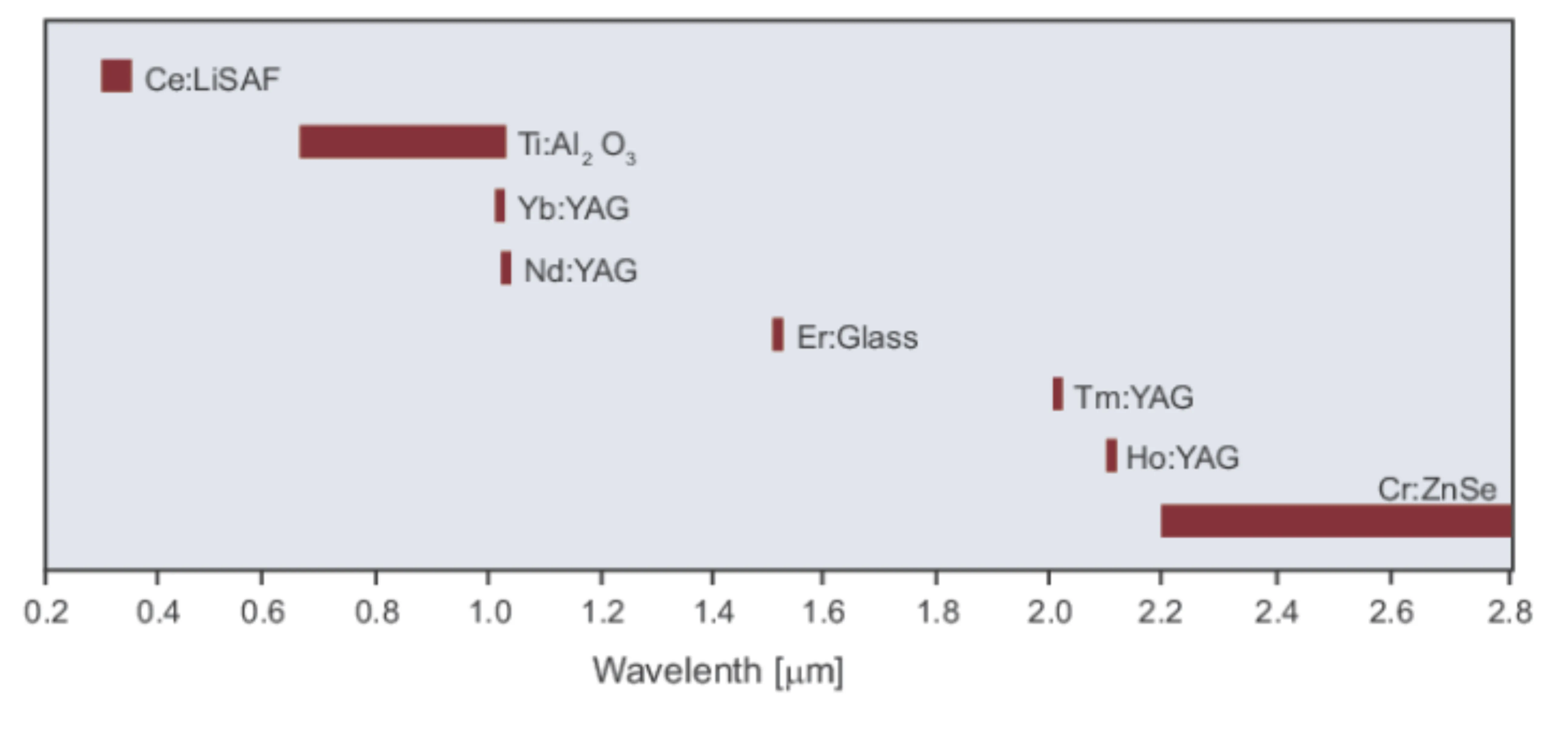
Note that Ti:Al${}_2$O${}_3$ is the famous Titanium-doped sapphire (Ti:sapphire) laser crystal. Its extremely broad emission bandwidth is due to the strong coupling of the active Ti${}^{3+}$ ion's d-orbitals to the crystal lattice vibrations (vibronic broadening). This broad bandwidth supports wide frequency tuning as a continuous-wave laser or the generation of ultrashort (femtosecond) pulses when mode-locked. It operates as a four-level (or quasi-three-level at the short wavelength end) laser system: