Table of Contents

7.1 Spherical Mirror Resonator
7.2 Resonance Frequencies
7.3 Resonator Losses

7 Optical Resonators

An optical resonator, or optical cavity, is a device designed to confine light, effectively storing electromagnetic energy within a defined volume for a certain duration. This is generally achieved by guiding the propagation of light along a path that self-reproduces after periodic round trips. One example of an optical resonator that we have already encountered is the Fabry-Pérot cavity.

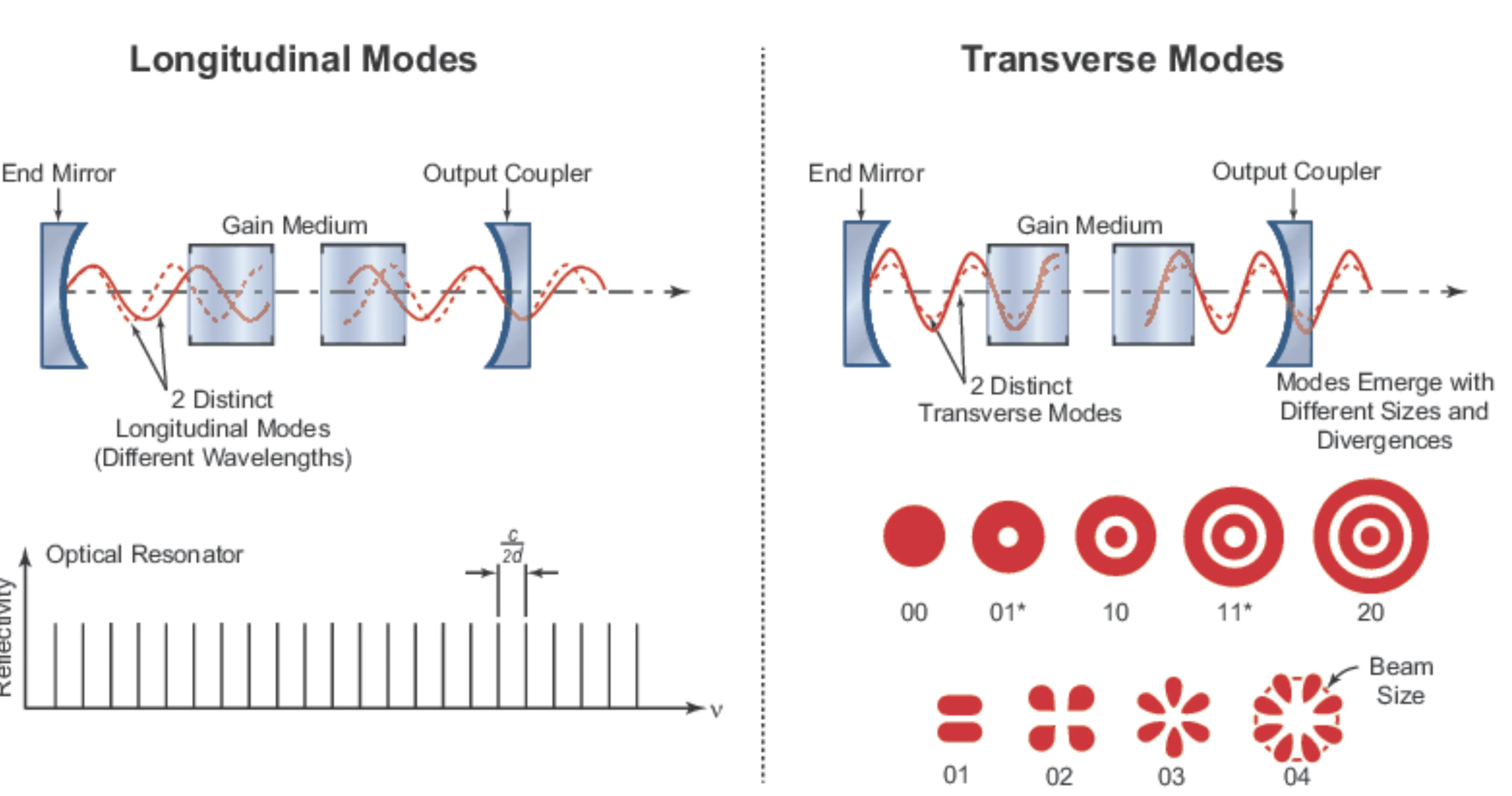
Optical resonators only allow discrete frequencies of light to be sustained and stored within them; these specific frequencies correspond to the longitudinal modes (or axial modes) of the resonator. Associated with these longitudinal modes are specific transverse intensity patterns, known as transverse modes. Most laser resonators are designed to support a specific fundamental transverse spatial beam shape, commonly a Gaussian beam:

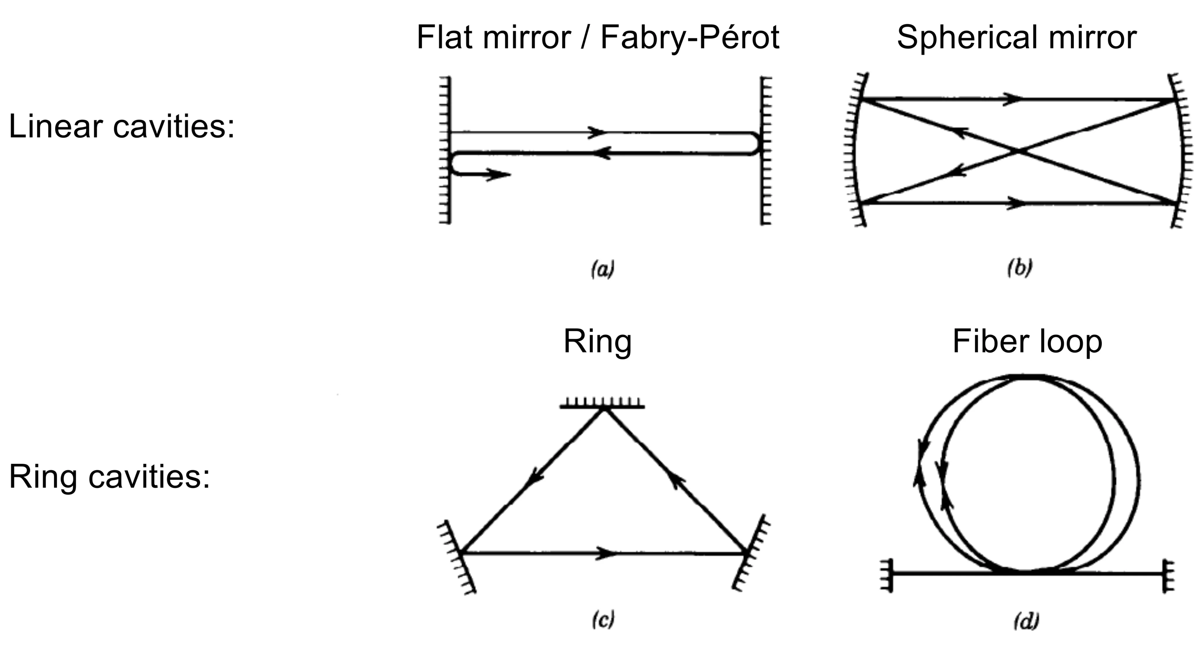
Attachments/Notes/2025 Quantum Electronics/7 Optical Resonators/03_Beams_and_resonators 4.webp|700

A very important concept is that of an optical mode, which, in broad terms, is a self-consistent electromagnetic field configuration that reproduces itself after one round trip within the resonator (apart from a possible constant phase shift and amplitude reduction due to losses). Modes are therefore eigensolutions of the wave equation subject to the boundary conditions imposed by the resonator geometry. In the following sections, we will mostly focus on linear cavities (formed by two mirrors). Ring resonators, which employ three or more mirrors to form a closed loop path, will also be mentioned, but their detailed treatment is more involved:

Attachments/Notes/2025 Quantum Electronics/7 Optical Resonators/03_Beams_and_resonators 5.webp|700

7.1 Spherical Mirror Resonator

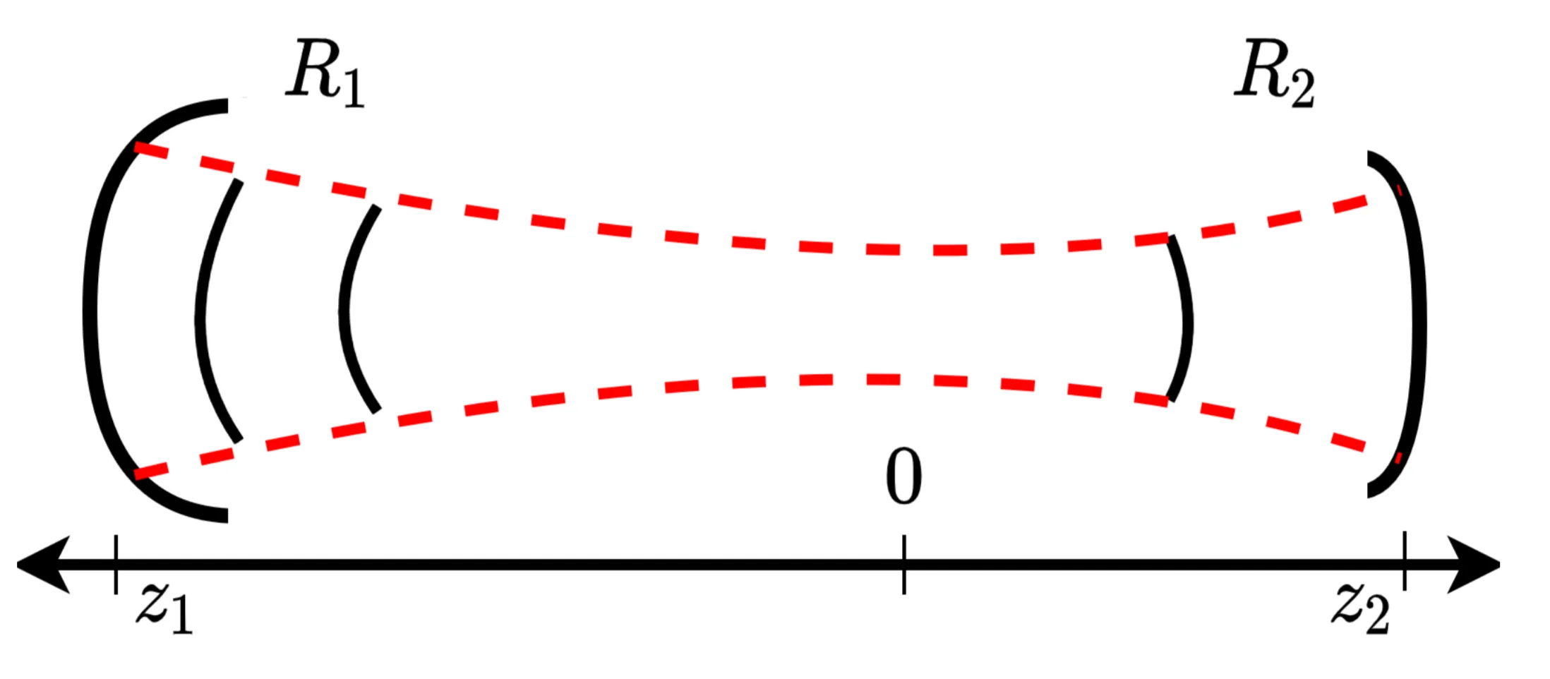
A spherical mirror resonator consists of two mirrors, both of which typically have spherically curved surfaces. As we will see later, this type of resonator generally offers much higher stability against misalignment compared to planar-mirror resonators (which are a special case of spherical mirrors with infinite radius of curvature). The following figure shows an example of a spherical mirror resonator with two concave mirrors:

Attachments/Notes/2025 Quantum Electronics/7 Optical Resonators/QE_script 4.webp|700

In this context, "spherical" means that the mirror surface is a segment of a sphere with a radius of curvature $R$ . The convention used here is that a positive $R$ denotes a concave mirror (curved towards the cavity interior), while a negative $R$ denotes a convex mirror. Some sources use the opposite sign convention, which is something one should always be aware of. We are interested in answering the question: "Under what conditions is the resonator stable?"

What does stability mean in this context? For an optical resonator, stability implies that the geometry allows a light beam (specifically, a paraxial Gaussian beam) to be confined and to replicate its transverse profile after each round trip, ignoring losses for now. A resonator is called stable if a paraxial ray, initially close to and slightly inclined to the optical axis, remains confined near the axis after an infinite number of round trips. Alternatively, using Gaussian beam optics, a resonator is stable if it supports a self-consistent Gaussian beam mode whose parameters (waist size and position) are physically realisable. From our discussion on paraxial ray optics and Gaussian beam optics, it should be clear that these two approaches (ray optics and Gaussian beam q-parameter transformation) are equivalent, as both use the same ABCD ray-transfer matrices.

The ray-transfer matrix for one complete round trip through the resonator, starting just after mirror 1, propagating a distance $d$ to mirror 2, reflecting from mirror 2, propagating distance $d$ back to mirror 1, and reflecting from mirror 1, is given by the product:

M_{RT} = (\begin{array}{ll} A & B \\ C & D \end{array}) = (\begin{array}{cc} 1 & 0 \\ - 1 / f_{1} & 1 \end{array}) (\begin{array}{cc} 1 & d \\ 0 & 1 \end{array}) (\begin{array}{cc} 1 & 0 \\ - 1 / f_{2} & 1 \end{array}) (\begin{array}{ll} 1 & d \\ 0 & 1 \end{array}),

where $f_{i} = R_{i} / 2$ is the focal length of mirror $i$ . Substituting $- 1 / f_{i} = - 2 / R_{i}$ :

M_{RT} = (\begin{array}{cc} 1 - \frac{2 d}{R_{2}} & 2 d (1 - \frac{d}{R_{2}}) \\ - 2 (\frac{1}{R_{1}} + \frac{1}{R_{2}} - \frac{2 d}{R_{1} R_{2}}) & (1 - \frac{2 d}{R_{1}}) (1 - \frac{2 d}{R_{2}}) - \frac{2 d}{R_{1}} \end{array}) .

The condition for a stable resonator is that a Gaussian beam can replicate its complex q-parameter after one round trip: $q_{2} = (A q_{1} + B) / (C q_{1} + D)$ must yield $q_{2} = q_{1} \equiv q$ . This leads to a quadratic equation for $q$ : $C q^{2} + (D - A) q - B = 0$ .
For a physically meaningful Gaussian beam, $q$ must be complex ( $q = (z - z_{w}) + i z_{R}$ with $z_{R} > 0$ ). This requires the discriminant of the quadratic equation for $q$ to be such that $q$ is complex, or more directly, the stability criterion derived from the ABCD matrix elements is:

- 1 < \frac{A + D}{2} < 1.

Using the elements of $M_{RT}$ , $(A + D) / 2 = 2 (1 - d / R_{1}) (1 - d / R_{2}) - 1 = 2 g_{1} g_{2} - 1$ .
The stability criterion then becomes $- 1 < 2 g_{1} g_{2} - 1 < 1$ , which simplifies to:

0 < g_{1} g_{2} < 1,

where $g_{i} = 1 - d / R_{i}$ is the g-parameter for mirror $i$ . Note that configurations where $g_{1} g_{2} = 0$ or $g_{1} g_{2} = 1$ are on the boundary of stability and are termed conditionally stable. In practice, these are difficult to achieve perfectly due to alignment tolerances and mirror imperfections. For instance, a Fabry-Pérot etalon with two perfectly plane mirrors ( $R_{1}, R_{2} \to \infty ⟹ g_{1} = g_{2} = 1$ ) is conditionally stable; only an ideally collimated on-axis beam would be confined, which is unrealistic. Such cavities are less efficient at storing light over many round trips than truly stable cavities.
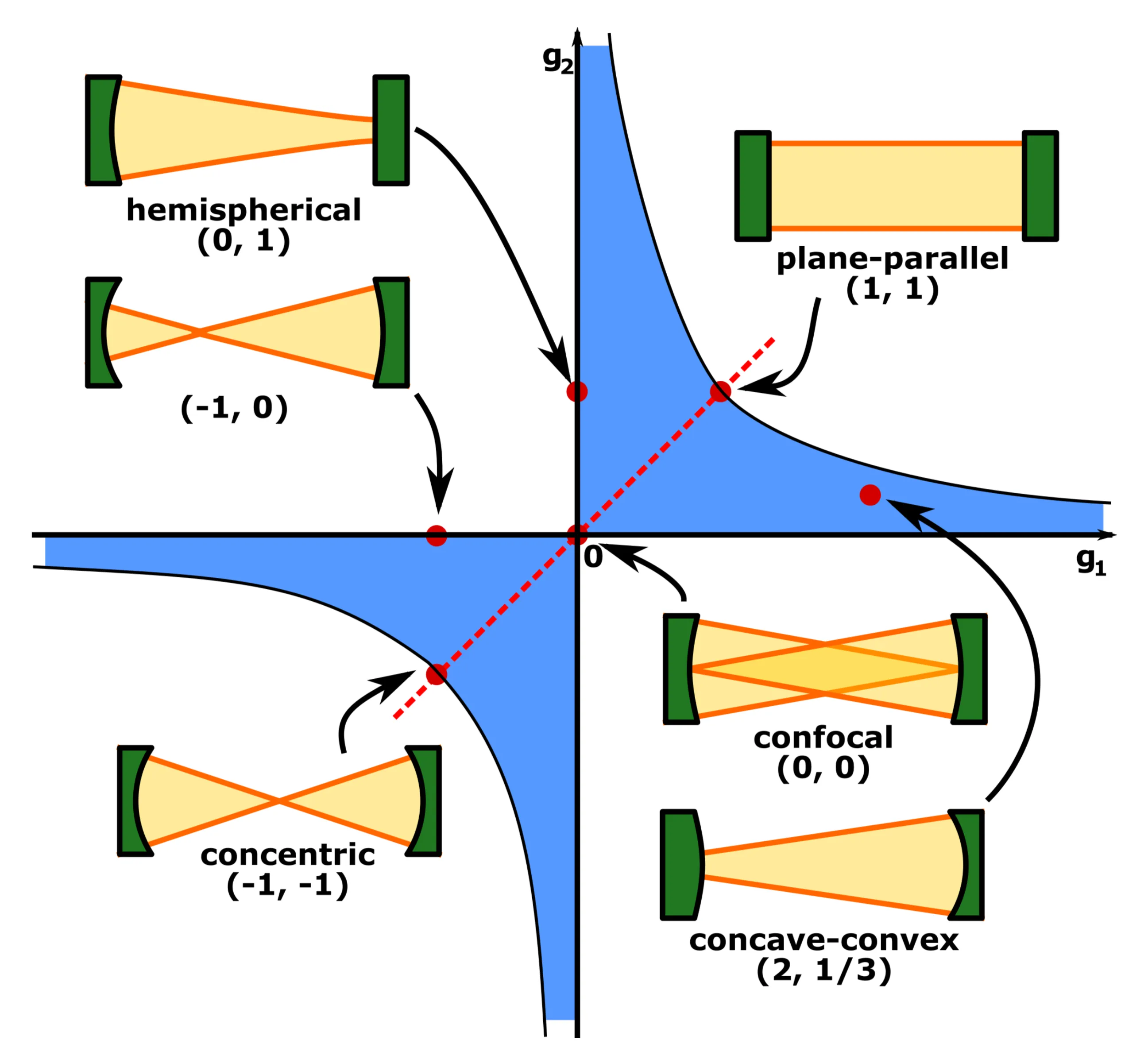
The stability map shows regions of stability (blue) based on $g_{1}$ and $g_{2}$ :

Attachments/Notes/2025 Quantum Electronics/7 Optical Resonators/QE_script 5.webp|700

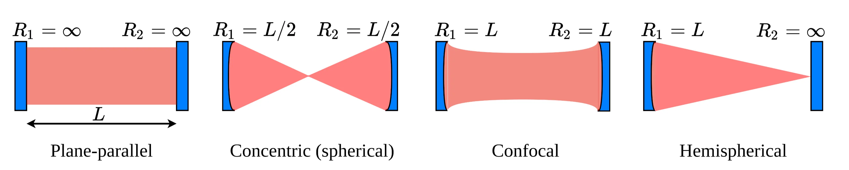
The dashed diagonal red line indicates symmetric configurations where $R_{1} = R_{2}$ (so $g_{1} = g_{2}$ ). Some typical stable configurations for spherical resonators are shown below:

Attachments/Notes/2025 Quantum Electronics/7 Optical Resonators/QE_script 6.webp|700

A resonator is symmetric if $R_{1} = R_{2}$ . A symmetric confocal resonator has $R_{1} = R_{2} = d$ (focal points of mirrors coincide at cavity centre). A symmetric concentric resonator has $R_{1} = R_{2} = d / 2$ (centres of curvature coincide), which is conditionally stable ( $g_{1} g_{2} = 1$ ).

A useful geometric stability test (attributed to Boyd and Kogelnik) relates to the overlap of the regions "covered" by each mirror as seen from the focal point of the other mirror. A more common statement is that a cavity is stable if the mirrors "see" each other through their focal points, meaning the focal point of one mirror lies within the cavity as seen from the other, and vice versa for certain configurations.

For a stable resonator, the self-consistent q-parameter implies that the wavefront curvature $R (z)$ of the Gaussian beam matches the curvature of the mirror at each mirror surface. For mirror 1 (the reference plane for the round trip), $1 / R (z_{1}) = 1 / R_{1}$ . The q-parameter solution gives $1 / R = (D - A) / (2 B)$ . The position of the beam waist $z_{w}$ (relative to mirror 1, say) and the Rayleigh range $z_{R} = Im [q]$ can also be determined:

z_{w 1} = Re [q_{1}] = \frac{d (R_{2} - d)}{R_{1} + R_{2} - 2 d}, (distance of waist from mirror 1)

z_{R}^{2} = (Im [q_{1}])^{2} = \frac{d (R_{1} - d) (R_{2} - d) (R_{1} + R_{2} - d)}{(R_{1} + R_{2} - 2 d)^{2}} .

7.1.1 Symmetric Spherical Mirror Resonators

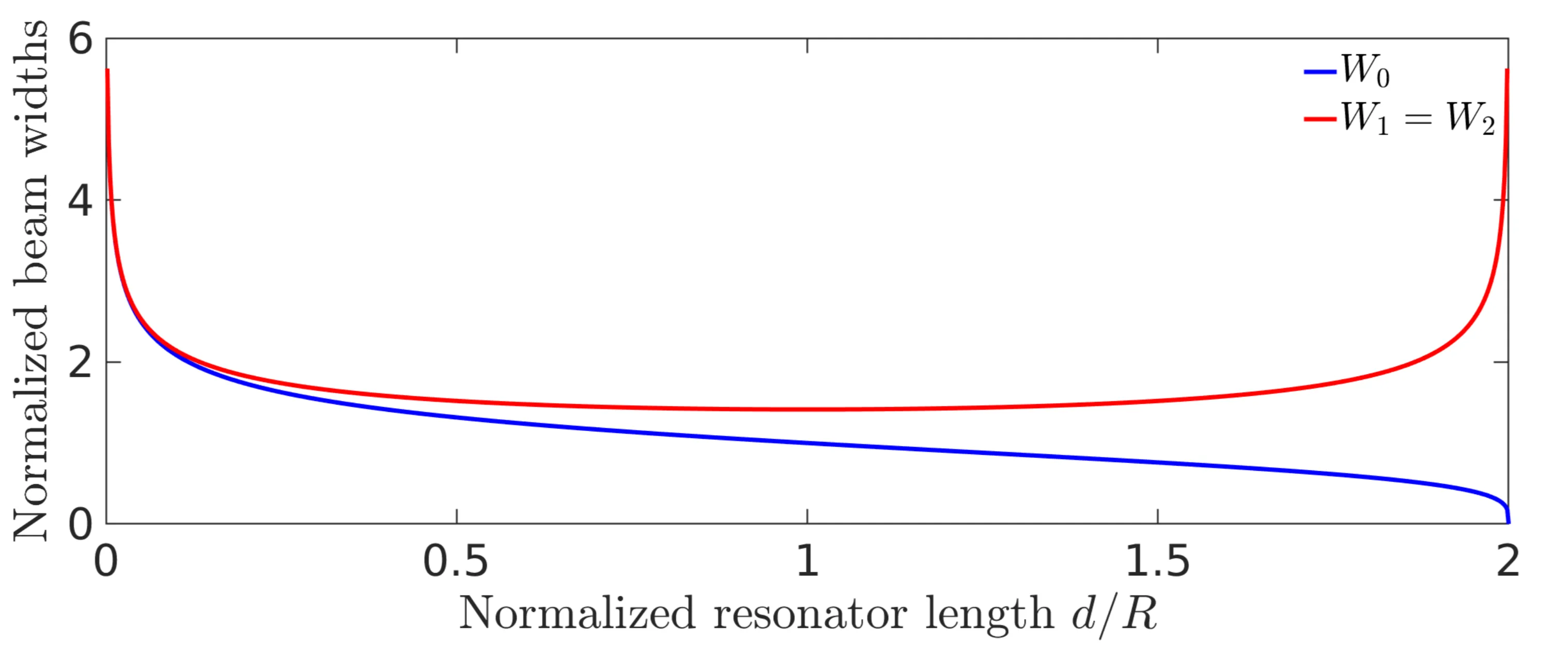
Consider the important case of a symmetric resonator where $R_{1} = R_{2} \equiv R$ . The stability criterion $0 < g_{1} g_{2} < 1$ becomes $0 < (1 - d / R)^{2} < 1$ . Since $(1 - d / R)^{2} \geq 0$ , this simplifies to $(1 - d / R)^{2} < 1$ , which means $- 1 < 1 - d / R < 1$ (and $1 - d / R \neq 0$ ). This implies $0 < d / R < 2$ .
For this symmetric case, the beam waist is at the centre of the cavity ( $z_{w} = d / 2$ from either mirror). We additionally obtain:

\begin{matrix} z_{R} = \frac{d}{2} \sqrt{\frac{2 R}{d} - 1}, \\ W_{0}^{2} = \frac{λ_{0} d}{2 π n} \sqrt{\frac{2 R}{d} - 1}, \\ W_{1}^{2} = W_{2}^{2} = W (d / 2)^{2} = W_{0}^{2} (1 + {(\frac{d / 2}{z_{R}})}^{2}) = \frac{λ_{0} d}{π n} \frac{R / d}{\sqrt{\frac{2 R}{d} - 1}} . \end{matrix}

The beam radius is minimal ( $W_{0}$ ) at the centre. It is largest on the mirrors for $d \to 0$ or $d \to 2 R$ . For the confocal case ( $d = R$ ):

\begin{matrix} z_{R} = d / 2 = R / 2, \\ W_{0} = \sqrt{λ_{0} R / (2 π n)}, \\ W_{1} = W_{2} = \sqrt{2} W_{0} = \sqrt{λ_{0} R / (π n)} . \end{matrix}

Attachments/Notes/2025 Quantum Electronics/7 Optical Resonators/QE_script 7.webp|700

7.2 Resonance Frequencies

So far, we have considered the condition that the spatial envelope $A (r)$ of a Gaussian beam must be self-replicating after one round trip. This extends to the full electric field, including its rapidly oscillating phase. Recall the phase of a Gaussian beam (propagating along $z$ , waist at $z_{w} = 0$ ) is $ϕ (x, y, z) = k z - ζ (z) + k (x^{2} + y^{2}) / (2 R (z))$ , where $ζ (z) = \arctan (z / z_{R})$ is the Gouy phase.
For a self-consistent mode, the total phase change accumulated by the beam over one complete round trip must be an integer multiple of $2 π$ .
The phase change for propagation from mirror 1 (at $z_{1}$ ) to mirror 2 (at $z_{2} = z_{1} + d$ ) on-axis ( $x = y = 0$ ) is $Δ ϕ_{1 \to 2} = k (z_{2} - z_{1}) - (ζ (z_{2}) - ζ (z_{1})) = k d - Δ ζ_{1 \to 2}$ .
The round-trip phase change $Δ Φ_{RT}$ (from mirror 1, to mirror 2, back to mirror 1, without considering reflection phases at mirrors for now) is:

Δ Φ_{RT} = 2 k d - 2 Δ ζ_{round trip},

where $Δ ζ_{round trip} = (ζ (z_{2}) - ζ (z_{1})) + (ζ (z_{1}) - ζ (z_{2}))_{return path, can be complex}$ . More simply, $Δ ζ_{round trip}$ is the total accumulated Gouy phase shift over one round trip. For a stable cavity supporting Hermite-Gaussian modes $T E M_{l, m, q}$ or Laguerre-Gaussian modes $L G_{p, l, q}$ , the resonance condition is:

k (2 d) - (l + m + 1)_{HG} Δ ζ_{0} = q 2 π or k (2 d) - (2 p + | l | + 1)_{LG} Δ ζ_{0} = q 2 π,

where $q$ is the longitudinal mode integer, and $Δ ζ_{0} = ζ (z_{2}) - ζ (z_{1})$ is the single-pass Gouy phase difference between the mirrors (the values depend on waist position).

The resonance condition is $2 k d - (N_{t} + 1) Δ ζ_{RT} = 2 π q$ , where $N_{t} = l + m$ or $2 p + | l |$ and $Δ ζ_{RT}$ is the round-trip Gouy phase.
Assuming $k = 2 π f n / c$ , the resonance frequencies $f_{q, l, m}$ are:

f_{q, l, m} = \frac{c}{2 n d} (q + (l + m + 1) \frac{Δ ζ_{RT}}{2 π}) .

The free spectral range (FSR) for longitudinal modes ( $l, m$ fixed) is $f_{F} = c / (2 n d)$ . The frequencies are approximately equally spaced by $f_{F}$ , with a small shift dependent on the transverse mode orders $(l, m)$ due to the Gouy phase. This means different transverse modes generally have slightly different resonance frequencies.

7.3 Resonator Losses

Up until now, we have treated resonators as perfect, implying, for instance, that mirrors have 100% reflectivity and there are no diffraction losses. In reality, losses are always present. Imperfect reflectivity is often the dominant loss mechanism and is, in fact, desired for one mirror to act as an output coupler. Losses broaden the resonance lines.

Consider an initial on-axis electric field amplitude $U_{0}$ inside the cavity just after a reference plane. After $j$ round trips, the field amplitude becomes:

U_{j} = r_{RT}^{j} U_{0} e^{i j Δ Φ_{RT}},

where $r_{RT}$ is the net amplitude reflectivity per round trip ( $0 < r_{RT} < 1$ ), and $Δ Φ_{RT}$ is the round-trip phase change (excluding the $2 π q$ part). If the cavity is continuously excited (or contains a gain medium), the total stored electric field $U$ is the sum of contributions from all preceding round trips:

U = U_{0} + r_{RT} U_{0} e^{i Δ Φ_{RT}} + r_{RT}^{2} U_{0} e^{i 2 Δ Φ_{RT}} + \dots = U_{0} \sum_{j = 0}^{\infty} {(r_{RT} e^{i Δ Φ_{RT}})}^{j} .

Using the formula for a geometric series, this sums to:

U = \frac{U_{0}}{1 - r_{RT} e^{i Δ Φ_{RT}}} .

The intracavity intensity $I \sim | U |^{2}$ . This can be rewritten (using $Δ Φ_{RT} \approx 2 π (f / f_{F}) - Gouy term$ ) as the Airy function, similar to the Fabry-Pérot interferometer transmittance:

I (f) = \frac{I_{circ,max}}{1 + {(\frac{2 F}{π})}^{2} \sin^{2} (Δ Φ_{RT} (f) / 2)},

where $I_{circ,max} = \frac{I_{0}}{(1 - r_{RT})^{2}}$ (if $I_{0}$ is related to input power coupled in per round trip), and the finesse $F$ is:

F = \frac{π \sqrt{r_{RT}}}{1 - r_{RT}} .

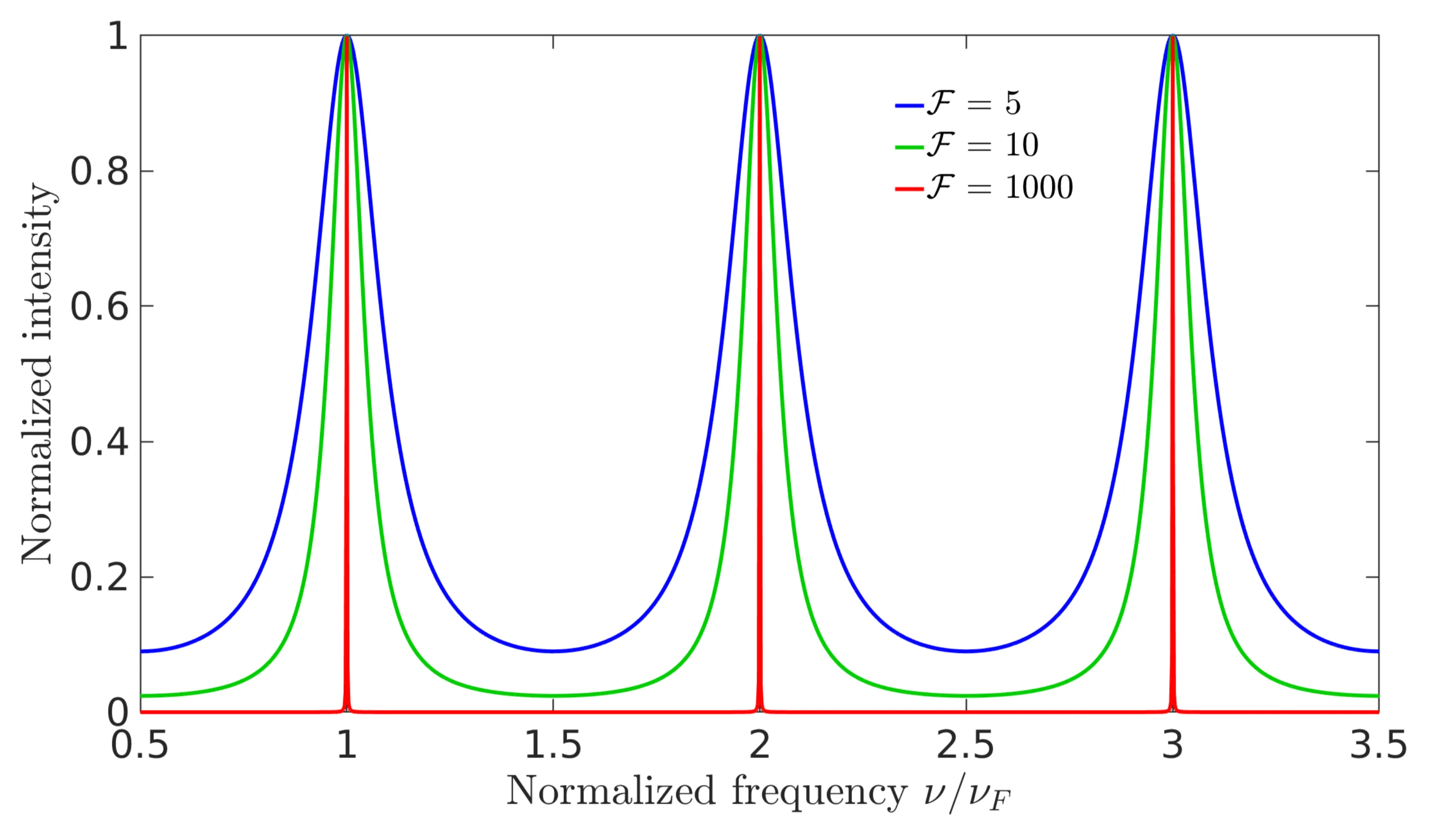
The next figure shows the normalised intensity spectrum of an optical resonator:

Attachments/Notes/2025 Quantum Electronics/7 Optical Resonators/QE_script 4-1.webp|700

The finesse $F$ controls the sharpness (linewidth) of the resonance peaks. Higher reflectivity $r_{RT}$ (lower loss) leads to higher finesse and sharper peaks. The Full Width at Half Maximum (FWHM) linewidth $δ f$ of each resonance is related to the free spectral range $f_{F}$ and the finesse by:

δ f = \frac{f_{F}}{F} .

Losses in a resonator can be characterised by an effective distributed loss coefficient $α_{loss}$ per unit length. If $L_{c}$ is the round-trip path length, the round-trip power reflectivity $R_{RT} = r_{RT}^{2}$ might be modelled as $R_{1} R_{2} e^{- 2 α_{loss} L_{c}}$ (where $R_{1}, R_{2}$ are mirror power reflectivities).
The finesse can then be expressed in terms of total round-trip losses. If round-trip power loss is small ( $1 - r_{RT}^{2} ≪ 1$ ), then $1 - r_{RT} \approx (1 - r_{RT}^{2}) / 2$ . For instance, if losses are primarily due to mirror transmission $T_{m} \approx 1 - r_{RT}$ , then $F \approx π / T_{m}$ (for high $r_{RT}$ ).
Then $F \approx π (1 - α_{r} d / 2) / (α_{r} d) \approx π / (α_{r} d)$ . This factor depends on whether $d$ is single path or round trip in $α_{r} d$ .

The quality factor $Q$ of a resonator mode is defined as $2 π$ times the ratio of stored energy to energy lost per optical cycle of the mode frequency $f_{q}$ :

Q = 2 π f_{q} \frac{Stored Energy}{Power Loss} = \frac{f_{q}}{δ f} .

Using $δ f = f_{F} / F$ , we obtain:

Q = F \frac{f_{q}}{f_{F}} .

Since $f_{q} \approx q f_{F}$ (where $q$ is a large integer for optical frequencies), the ratio $f_{q} / f_{F} \approx q$ is typically very large. Thus, the quality factor $Q$ is generally much larger than the finesse $F$ for optical resonators.