Jump back to chapter selection.

Table of Contents

6.1 Gaussian Beam Optics
6.2 Paraxial Helmholtz Equation and Slowly-Varying Envelope Approximation
6.3 Hermite-Gaussian Beams
6.4 Laguerre-Gaussian Beams
6.5 Bessel Beams
6.6 Summary

6 Beam Types

In this chapter, we return to the treatment of optical beams and will discuss different types of beams encountered in optics. The most important of these, particularly in laser applications, is the Gaussian beam.

6.1 Gaussian Beam Optics

Gaussian beams are highly relevant in optical laboratories as they accurately describe the spatial profile of light produced by most lasers operating in the fundamental transverse mode, and they are the characteristic modes of stable optical resonators and cavities. A fundamental Gaussian beam with its waist (narrowest point) located at $z = 0$ and propagating along the $z$ -axis is described by the complex amplitude $U (r)$ :

U (r) = A_{0} \frac{W_{0}}{W (z)} \exp (- \frac{ρ^{2}}{W^{2} (z)}) \exp (- i k z - i k \frac{ρ^{2}}{2 R (z)} + i ζ (z)),

where $ρ^{2} = x^{2} + y^{2}$ is the transverse radial distance from the beam axis. The beam is characterised by the following parameters:

\begin{aligned} Beam Radius at distance z : & W (z) & = W_{0} \sqrt{1 + {(\frac{z}{z_{R}})}^{2}}, \\ Radius of Curvature of wavefronts at z : & R (z) & = z [1 + {(\frac{z_{R}}{z})}^{2}], \\ Gouy Phase Shift at z : & ζ (z) & = \arctan (\frac{z}{z_{R}}), \\ Beam Waist Radius (at z = 0) : & W_{0} & (a fundamental parameter), \\ Rayleigh Range: & z_{R} & = \frac{π W_{0}^{2} n}{λ_{0}} = \frac{k W_{0}^{2}}{2}, \\ Far-field Half-Angle of Divergence: & θ_{0} & \approx \frac{W_{0}}{z_{R}} = \frac{λ_{0}}{π W_{0} n} . \end{aligned}

Here, $λ_{0}$ is the vacuum wavelength, $n$ is the refractive index of the medium, and $k = 2 π n / λ_{0}$ is the wave number in the medium.

These parameters are explained further in the following subsections.

6.1.1 Gaussian Beams as Solution to the Helmholtz Equation

The Gaussian beam form $U (r) = A (r) e^{- i k z}$ (where $A (r)$ is a slowly varying complex envelope) is a solution to the paraxial Helmholtz equation. Starting with the Helmholtz equation for a scalar field $U (r)$ :

\nabla^{2} U + k^{2} U = 0.

Substituting $U (r) = A (x, y, z) e^{- i k z}$ and applying the slowly varying envelope approximation (SVEA), specifically neglecting $\frac{\partial^{2} A}{\partial z^{2}}$ compared to $k \frac{\partial A}{\partial z}$ (i.e., $| \frac{\partial^{2} A}{\partial z^{2}} | ≪ | 2 k \frac{\partial A}{\partial z} |$ ), transforms the Helmholtz equation into the paraxial Helmholtz equation:

\nabla_{T}^{2} A - 2 i k \frac{\partial A}{\partial z} = 0,

where $\nabla_{T}^{2} = \frac{\partial^{2}}{\partial x^{2}} + \frac{\partial^{2}}{\partial y^{2}}$ is the transverse Laplacian. A fundamental solution to this equation has the form:

A (x, y, z) = \frac{A_{1}}{q (z)} \exp (- i k \frac{x^{2} + y^{2}}{2 q (z)}) with q (z) = (z - z_{w}) + i z_{R} .

Here, $z_{w}$ is the position of the beam waist (if $z_{w} = 0$ , then $q (z) = z + i z_{R}$ ), and $A_{1}$ is a constant. This solution directly yields the Gaussian beam parameters.

$W (z)$ is the beam radius, defined as the radial distance where the beam intensity falls to $1 / e^{2}$ (approx. 13.5%) of its on-axis maximum value in a transverse plane at position $z$ . Twice the beam radius, $2 W (z)$ , is sometimes called the spot size. The transverse intensity profile of a Gaussian beam is circularly symmetric (for the fundamental mode).

Attachments/Notes/2025 Quantum Electronics/6 Beam Types/02_Fundamental_phenomena 25.webp|700

Here, the minimal beam radius (waist) $W_{0}$ occurs at the waist position (e.g., $z = 0$ if $z_{w} = 0$ ). From the waist, the radius $W (z)$ increases hyperbolically in both directions. Wavefronts are planar at the beam waist ( $R (z_{w}) \to \infty$ ) but become increasingly curved (approximately spherical) far from the waist. For a fixed Rayleigh range $z_{R}$ , the waist radius $W_{0} = \sqrt{2 z_{R} / k} = \sqrt{λ_{0} z_{R} / (π n)}$ is smaller for shorter wavelengths $λ_{0}$ .

6.1.2 Rayleigh Length

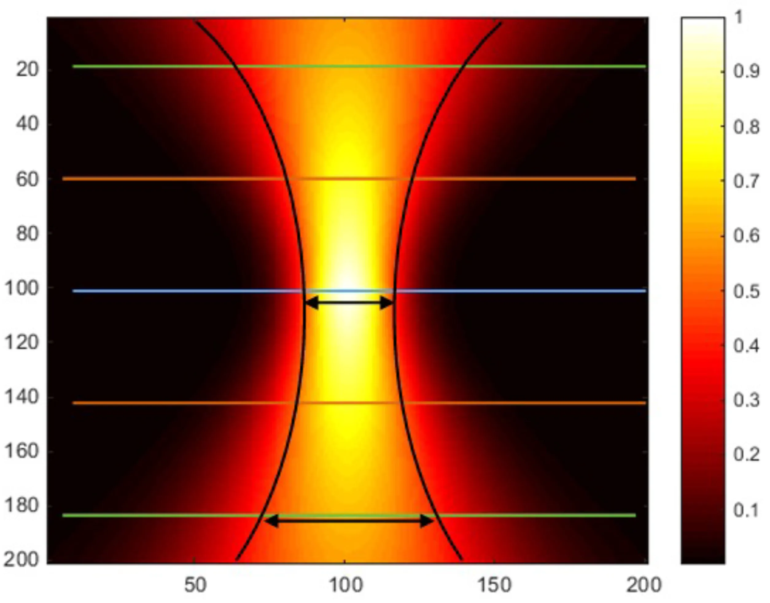
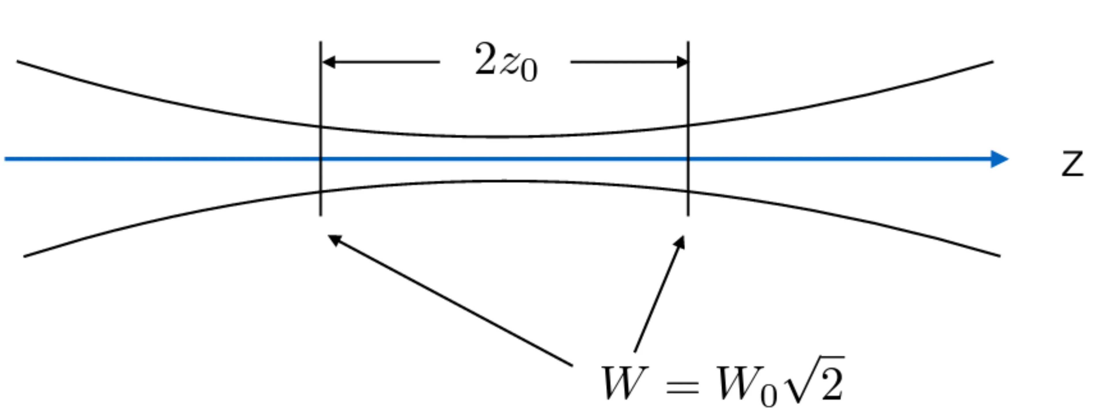
The Rayleigh range (or Rayleigh length) $z_{R}$ is a crucial parameter characterising the longitudinal extent of the beam waist region. It is defined as the distance from the waist ( $z = z_{w}$ ) at which the beam radius has increased to $W (z_{w} \pm z_{R}) = W_{0} \sqrt{2}$ , meaning the cross-sectional area of the beam, $π W^{2} (z)$ , has doubled compared to its area at the waist, $π W_{0}^{2}$ .

Attachments/Notes/2025 Quantum Electronics/6 Beam Types/02_Fundamental_phenomena 26.webp|700

The depth of focus of a Gaussian beam is often considered to be $2 z_{R}$ . We deduce the following behaviour:

For a fixed beam waist $W_{0}$ : The shorter the wavelength $λ_{0}$ (or larger $n$ ), the longer the Rayleigh range $z_{R} = π W_{0}^{2} n / λ_{0}$ , and thus the longer the depth of focus.
For a fixed wavelength $λ_{0}$ : The larger the beam waist $W_{0}$ , the longer the Rayleigh range $z_{R}$ and depth of focus.

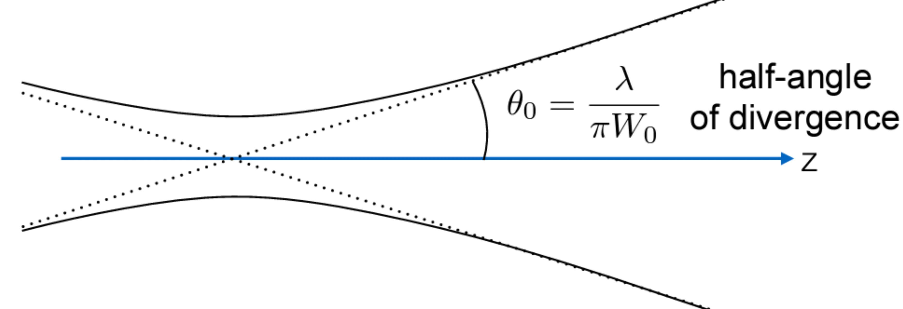
6.1.3 Beam Divergence

The beam divergence describes how quickly the beam width $W (z)$ increases for $| z | ≫ z_{R}$ (in the far field). The half-angle of divergence $θ_{0}$ is defined as the angle of the asymptote of $W (z)$ with respect to the $z$ -axis:

θ_{0} = lim_{z \to \infty} \frac{W (z)}{| z - z_{w} |} \approx \frac{W_{0}}{z_{R}} = \frac{λ_{0}}{π W_{0} n} .

Attachments/Notes/2025 Quantum Electronics/6 Beam Types/02_Fundamental_phenomena 27.webp|700

Again, we deduce the following behaviour:

For a fixed beam waist $W_{0}$ : The shorter the wavelength $λ_{0}$ , the smaller the divergence angle $θ_{0}$ .
For a fixed wavelength $λ_{0}$ : The larger the beam waist $W_{0}$ , the smaller the divergence angle $θ_{0}$ . This is a manifestation of diffraction: a more spatially confined beam (smaller $W_{0}$ ) diffracts more rapidly (larger $θ_{0}$ ).

6.1.4 Wavefront of Gaussian Beams

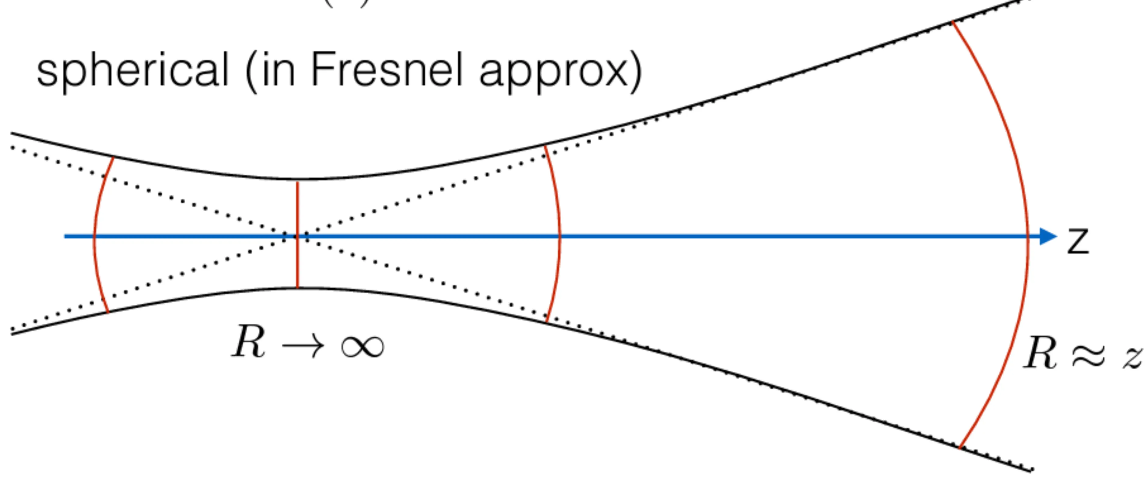
The radius of curvature $R (z)$ of the wavefronts of a Gaussian beam is given by:

R (z) = (z - z_{w}) [1 + {(\frac{z_{R}}{z - z_{w}})}^{2}] .

Near the beam waist ( $z \approx z_{w}$ ), $R (z_{w}) \to \infty$ , indicating planar wavefronts. Far from the waist ( $| z - z_{w} | ≫ z_{R}$ ), $R (z) \approx z - z_{w}$ , meaning the wavefronts become approximately spherical, appearing to originate from a point source located at the waist position $z_{w}$ .

Attachments/Notes/2025 Quantum Electronics/6 Beam Types/02_Fundamental_phenomena 28.webp|700

6.1.5 Gouy Phase

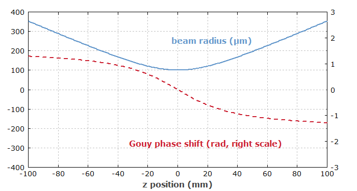
The term $ζ (z) = \arctan (\frac{z - z_{w}}{z_{R}})$ in the phase of the Gaussian beam is the Gouy phase shift (figure source):

Attachments/Notes/2025 Quantum Electronics/6 Beam Types/Pasted image 20250331190810.png|700

The Gouy phase varies from $- π / 2$ for $z ≪ - z_{R}$ (relative to $z_{w}$ ) through $0$ at the waist $z = z_{w}$ , to $+ π / 2$ for $z ≫ z_{R}$ . The limits are:

\begin{aligned} (z - z_{w}) \to \infty & ⟹ ζ (z) \to π / 2 \\ (z - z_{w}) \to - \infty & ⟹ ζ (z) \to - π / 2. \end{aligned}

The Gouy phase represents an additional axial phase shift experienced by a focused Gaussian beam compared to an ideal plane wave (or a spherical wave originating from a point focus). This phase shift is a consequence of the transverse confinement of the beam; as the beam passes through its focus, it accumulates this extra phase. It is significant only in the region around the beam waist, over a range of approximately $\pm z_{R}$ .

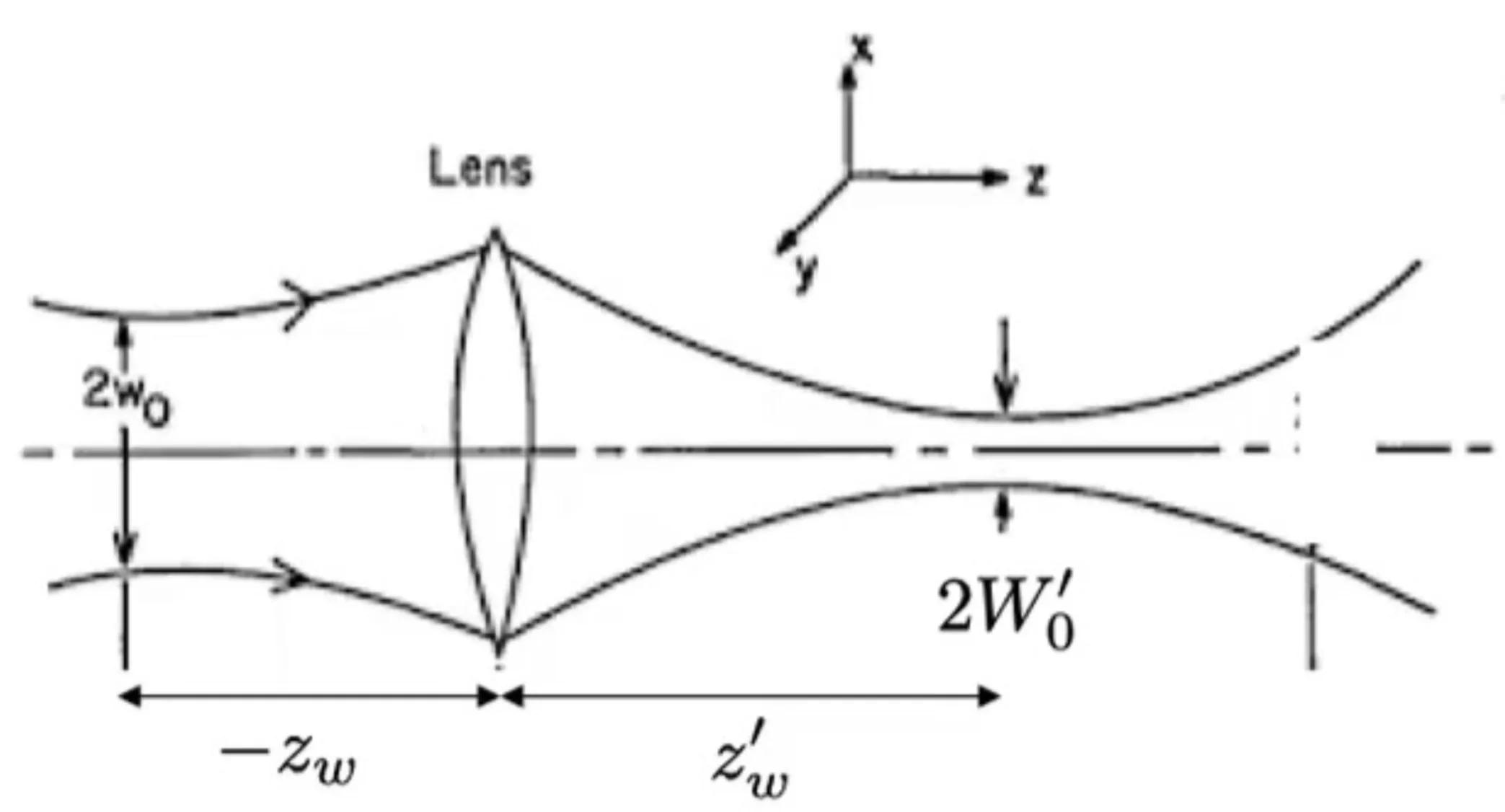
6.1.6 Shifting the Gaussian Beam (Transformation by a Thin Lens)

We can define the Gaussian beam with its waist at an arbitrary position $z = z_{w}$ . When such a beam passes through a thin lens of focal length $f$ located at, say, $z = z_{L}$ , the lens transforms the beam parameters. The radius of curvature of the wavefront changes according to the lensmaker's formula for wavefronts (assuming the lens is at $z = 0$ for simplicity of this formula, and input $R_{i n}$ gives output $R_{o u t}$ ):

\frac{1}{R_{out}} = \frac{1}{R_{in}} - \frac{1}{f} .

The beam waist radius $W$ is unchanged immediately after passing through an ideal thin lens: $W_{out} (z_{L}) = W_{in} (z_{L})$ .

Attachments/Notes/2025 Quantum Electronics/6 Beam Types/02_Fundamental_phenomena 30.webp|700
(Figure shows transformation of $W (z)$ and $R (z)$ by a lens)

If a Gaussian beam with waist $W_{0}$ at $z_{w}$ (input parameters $z_{R}, W_{0}$ ) is incident on a thin lens of focal length $f$ , the output beam will be a new Gaussian beam with a new waist $W_{0}^{'}$ at a new position $z_{w}^{'}$ , and a new Rayleigh range $z_{R}^{'}$ . These new parameters can be found using the ABCD matrix formalism for the q-parameter. The magnification $M = W_{0}^{'} / W_{0}$ and the new waist position can be expressed in terms of $f$ , $z_{w}$ (distance of input waist from lens), and $z_{R}$ . For a lens at $z = 0$ , and input waist at $z_{1}$ (so $z_{w} = z_{1}$ in prior notation), the output waist is at $z_{2}$ and has radius $W_{02}$ :

New Rayleigh range: $z_{R 2} = M^{2} z_{R 1}$ .
New waist radius: $W_{02} = M W_{01}$ .
Magnification: $M = \frac{| f |}{\sqrt{(z_{1} + f)^{2} + z_{R 1}^{2}}}$ .
New waist position: $z_{2} - f = - M^{2} (z_{1} + f)$ .

The new waist radius is $M W_{01}$ , and the new Rayleigh range changes by $M^{2}$ .

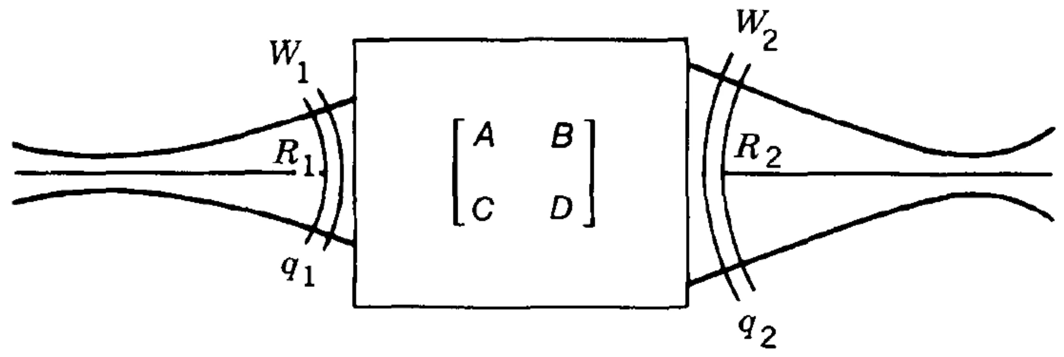
6.1.7 ABCD Law for Gaussian Beams

The propagation of Gaussian beams through paraxial optical systems can be conveniently described using the complex beam parameter (q-parameter), defined as:

q (z) = (z - z_{w}) + i z_{R} .

Alternatively, its inverse is related to the radius of curvature $R (z)$ and beam radius $W (z)$ :

\frac{1}{q (z)} = \frac{1}{R (z)} - i \frac{λ_{0}}{π n W^{2} (z)} .

If an optical system is described by an ABCD ray-transfer matrix for paraxial rays, the q-parameter of an input Gaussian beam $q_{1}$ transforms to an output $q_{2}$ according to Kogelnik's ABCD law:

Attachments/Notes/2025 Quantum Electronics/6 Beam Types/02_Fundamental_phenomena 31.webp|700

q_{2} = \frac{A q_{1} + B}{C q_{1} + D} .

This powerful result allows us to use the same ABCD matrices derived for paraxial ray optics to transform Gaussian beams. For example:

Propagation through free space of length $d$ : $M = (\begin{matrix} 1 & d \\ 0 & 1 \end{matrix})$ .
$q_{2} = \frac{1 \cdot q_{1} + d}{0 \cdot q_{1} + 1} = q_{1} + d$ .
Passage through a thin lens of focal length $f$ : $M = (\begin{matrix} 1 & 0 \\ - 1 / f & 1 \end{matrix})$ .
$q_{2} = \frac{1 \cdot q_{1} + 0}{(- 1 / f) q_{1} + 1} = \frac{q_{1}}{1 - q_{1} / f}$ .
This connection between ray optics (via ABCD matrices) and Gaussian beam optics (via the q-parameter) is not coincidental. In the limit $λ_{0} \to 0$ , the imaginary part of $1 / q (z)$ vanishes, and $1 / q (z) \to 1 / R (z)$ . For paraxial rays, $R (z) \approx r (z) / θ (z)$ (where $r$ is ray height, $θ$ is ray angle). The ABCD law for $q$ then becomes consistent with the ray transformation $(\binom{r_{2}}{θ_{2}}) = M (\binom{r_{1}}{θ_{1}})$ .

6.2 Paraxial Helmholtz Equation and Slowly-Varying Envelope Approximation

Let us return once more to the Helmholtz equation, introduced in section 6.1.1:

\nabla^{2} U + k^{2} U = 0.

We seek solutions of the form $U (x, y, z) = A (x, y, z) e^{- i k z}$ , where $A (x, y, z)$ is a slowly varying complex envelope representing the deviation from a simple plane wave propagating along $z$ . Substituting this into the Helmholtz equation, we obtain:

(\nabla_{T}^{2} A + \frac{\partial^{2} A}{\partial z^{2}}) e^{- i k z} - 2 i k \frac{\partial A}{\partial z} e^{- i k z} - k^{2} A e^{- i k z} + k^{2} A e^{- i k z} = 0.

This simplifies to:

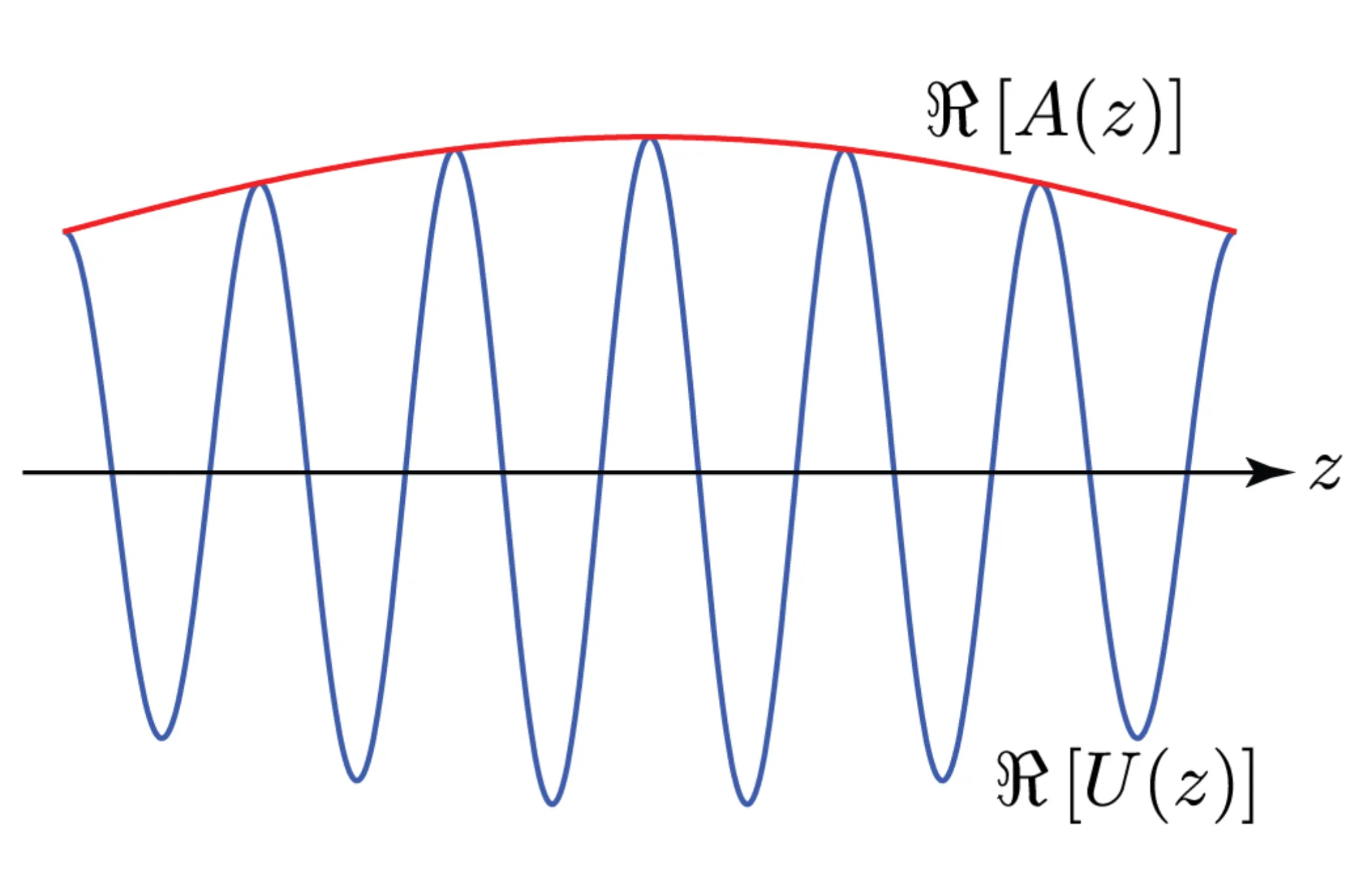
\nabla_{T}^{2} A + \frac{\partial^{2} A}{\partial z^{2}} - 2 i k \frac{\partial A}{\partial z} = 0.

We now apply the paraxial approximation, which is a form of the slowly-varying envelope approximation (SVEA) with respect to $z$ . We assume that the envelope $A$ changes much more slowly along $z$ than the fast phase oscillation $e^{- i k z}$ , and also that its transverse variations are slow. Specifically, we assume that the second derivative with respect to $z$ is much smaller than the term involving the first derivative:

| \frac{\partial^{2} A}{\partial z^{2}} | ≪ | k \frac{\partial A}{\partial z} | .

Under this condition, we can neglect the $\frac{\partial^{2} A}{\partial z^{2}}$ term, yielding the paraxial Helmholtz equation (or paraxial wave equation):

\nabla_{T}^{2} A - 2 i k \frac{\partial A}{\partial z} = 0, where \nabla_{T}^{2} = \frac{\partial^{2}}{\partial x^{2}} + \frac{\partial^{2}}{\partial y^{2}} .

The next figure schematically sketches the field (fast oscillations) and its slowly varying envelope.

Attachments/Notes/2025 Quantum Electronics/6 Beam Types/03_Beams_and_resonators.webp|700

Consider now the 2D spatial Fourier transform of the paraxial Helmholtz equation with respect to $x$ and $y$ . Let $B (k_{x}, k_{y}, z) = F_{x y} {A (x, y, z)}$ . Then $F_{x y} {\nabla_{T}^{2} A} = - (k_{x}^{2} + k_{y}^{2}) B$ . This yields:

- (k_{x}^{2} + k_{y}^{2}) B - 2 i k \frac{\partial B}{\partial z} = 0.

This is a first-order ordinary differential equation for $B$ with respect to $z$ :

\frac{\partial B}{\partial z} = \frac{i (k_{x}^{2} + k_{y}^{2})}{2 k} B .

The solution is:

B (k_{x}, k_{y}, z) = B (k_{x}, k_{y}, 0) \exp (i z \frac{k_{x}^{2} + k_{y}^{2}}{2 k}) .

This exactly retrieves the phase factor $e^{- i z (k_{x}^{2} + k_{y}^{2}) / (2 k)}$ found in the transfer function for Fresnel propagation (section 5.3) if we recall that $A$ is the envelope relative to $e^{- i k z}$ . The transfer function for $U$ was $H_{F r e s n e l} \approx e^{i k z} e^{- i z (k_{x}^{2} + k_{y}^{2}) / (2 k)}$ . The factor $e^{- i z (k_{x}^{2} + k_{y}^{2}) / (2 k)}$ here is the transfer function for the envelope $A$ .

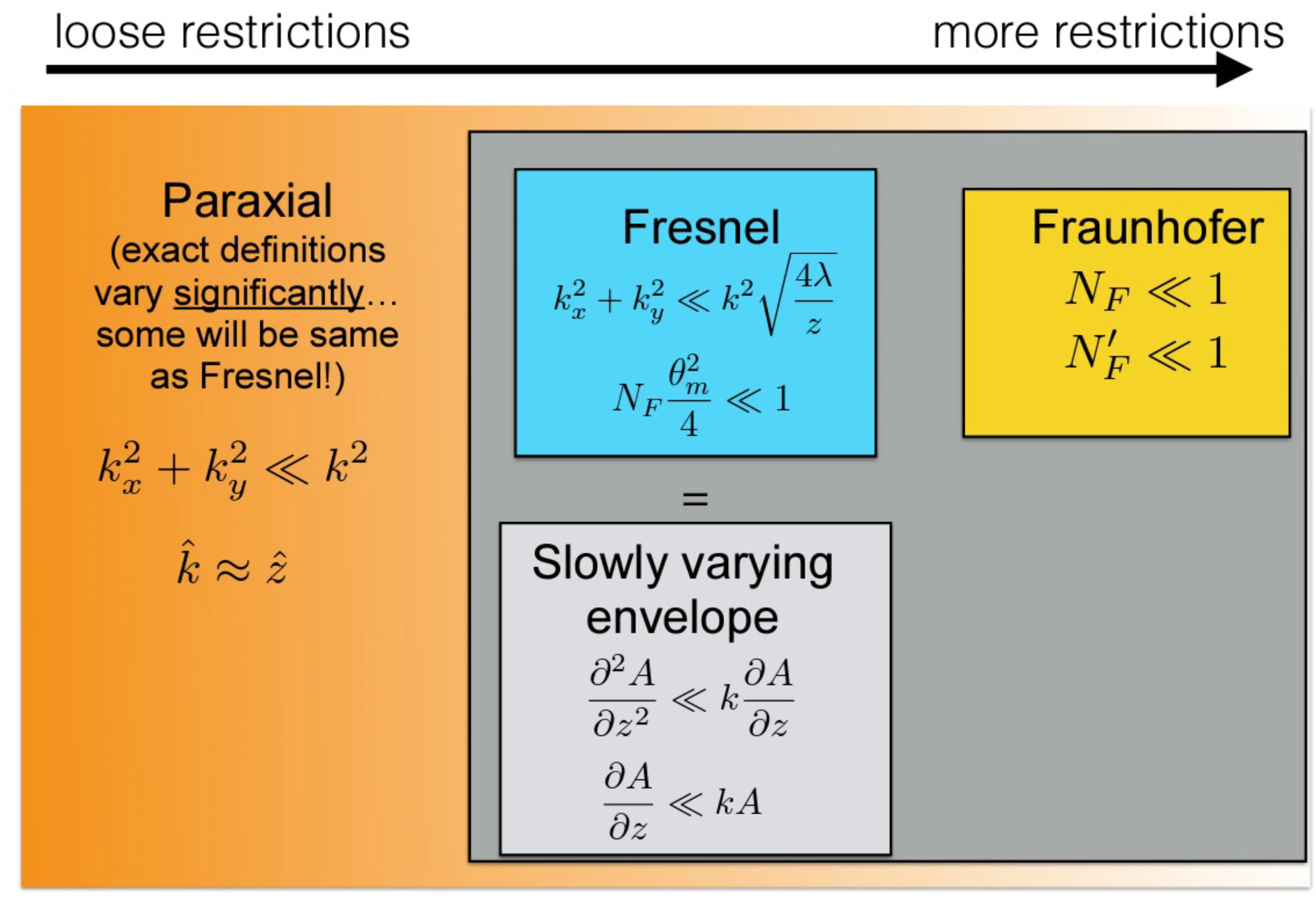
At this point, it is good to recall the hierarchy of approximations we have used:

Attachments/Notes/2025 Quantum Electronics/6 Beam Types/03_Beams_and_resonators 1.webp|700

6.3 Hermite-Gaussian Beams

This subsection and the remainder of this chapter will be kept rather concise, as it serves mainly to introduce these beam types rather than delve into exhaustive detail.

The fundamental Gaussian beam ( $T E M_{00}$ ) is not the only non-plane wave solution of the paraxial Helmholtz equation. Recall that the complex envelope of the fundamental Gaussian beam can be written as:

A_{G} (x, y, z) = \frac{A_{1}}{q (z)} \exp (- i k \frac{x^{2} + y^{2}}{2 q (z)}),

with $q (z) = (z - z_{w}) + i z_{R}$ . Higher-order solutions can be constructed by multiplying $A_{G} (x, y, z)$ by polynomials in $x$ and $y$ and an additional $z$ -dependent phase factor. We consider solutions of the form:

A (x, y, z) = X (\frac{\sqrt{2} x}{W (z)}) Y (\frac{\sqrt{2} y}{W (z)}) e^{i Z (z)} A_{G} (x, y, z),

where $X$ and $Y$ are real functions of scaled transverse coordinates, and $Z (z)$ is a real, slowly-varying phase function. Since $X$ and $Y$ are real, the phase fronts of these higher-order beams have approximately the same radius of curvature $R (z)$ as the fundamental Gaussian beam. This implies they behave similarly when incident on thin lenses and curved mirrors (within the paraxial approximation).

The solutions obtained in Cartesian coordinates are the Hermite-Gaussian beams, $U_{l, m} (x, y, z)$ . Their complex amplitude is given by:

\begin{aligned} U_{l, m} (x, y, z) = & C_{l, m} \frac{W_{0}}{W (z)} H_{l} (\frac{\sqrt{2} x}{W (z)}) H_{m} (\frac{\sqrt{2} y}{W (z)}) \exp (- \frac{x^{2} + y^{2}}{W^{2} (z)}) \\ \times \exp [- i k z - i k \frac{x^{2} + y^{2}}{2 R (z)} + i (l + m + 1) \arctan (\frac{z - z_{w}}{z_{R}})], \end{aligned}

where $C_{l, m}$ is a normalisation constant, $H_{l} (u)$ and $H_{m} (v)$ are Hermite polynomials of order $l$ and $m$ respectively. The term $G_{p} (u) = H_{p} (u) e^{- u^{2} / 2}$ is the Hermite-Gaussian function. The Gouy phase is now $(l + m + 1) \arctan ((z - z_{w}) / z_{R})$ .
The integers $l, m \geq 0$ are mode indices. The fundamental Gaussian beam corresponds to $l = m = 0$ .
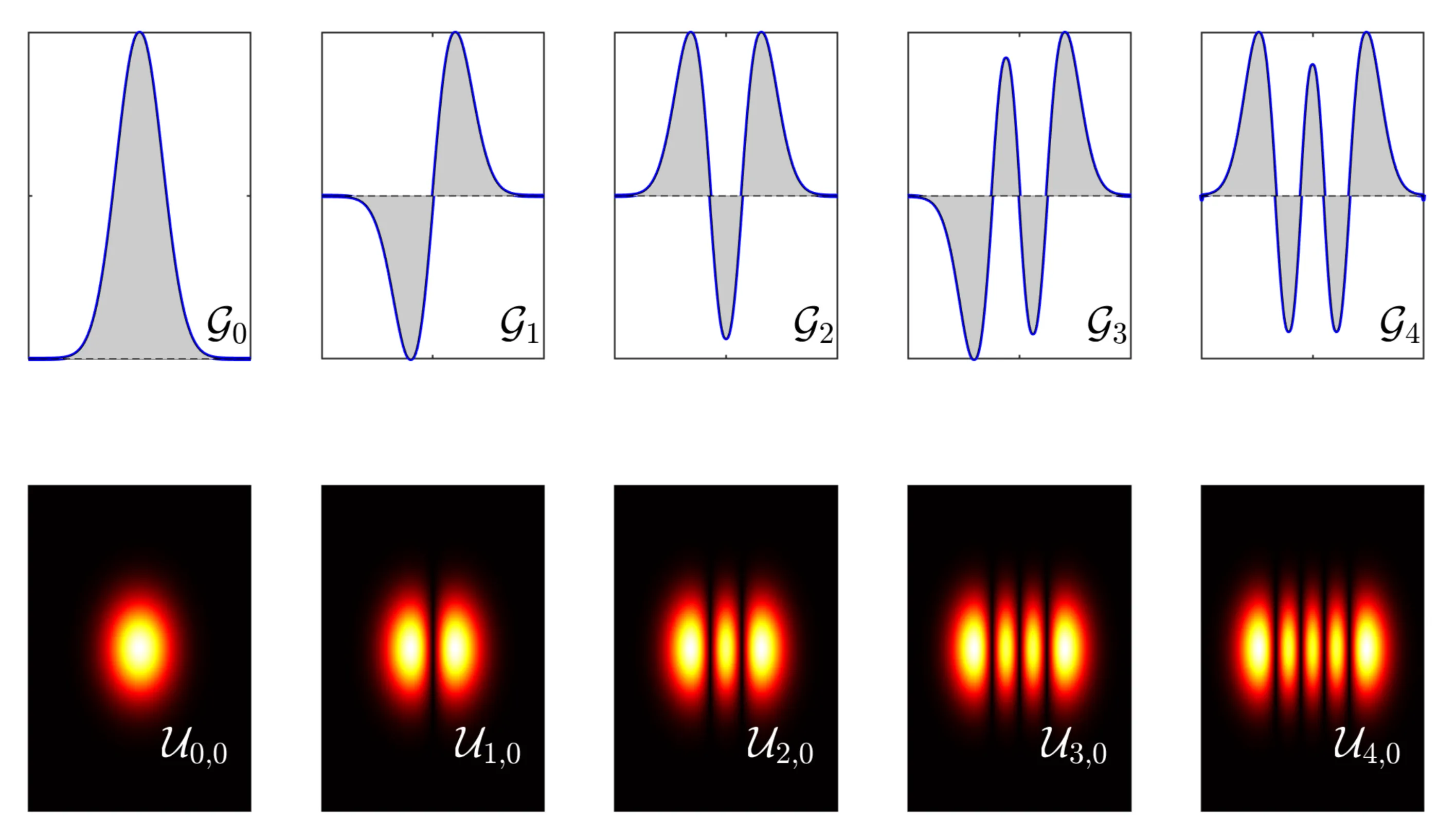
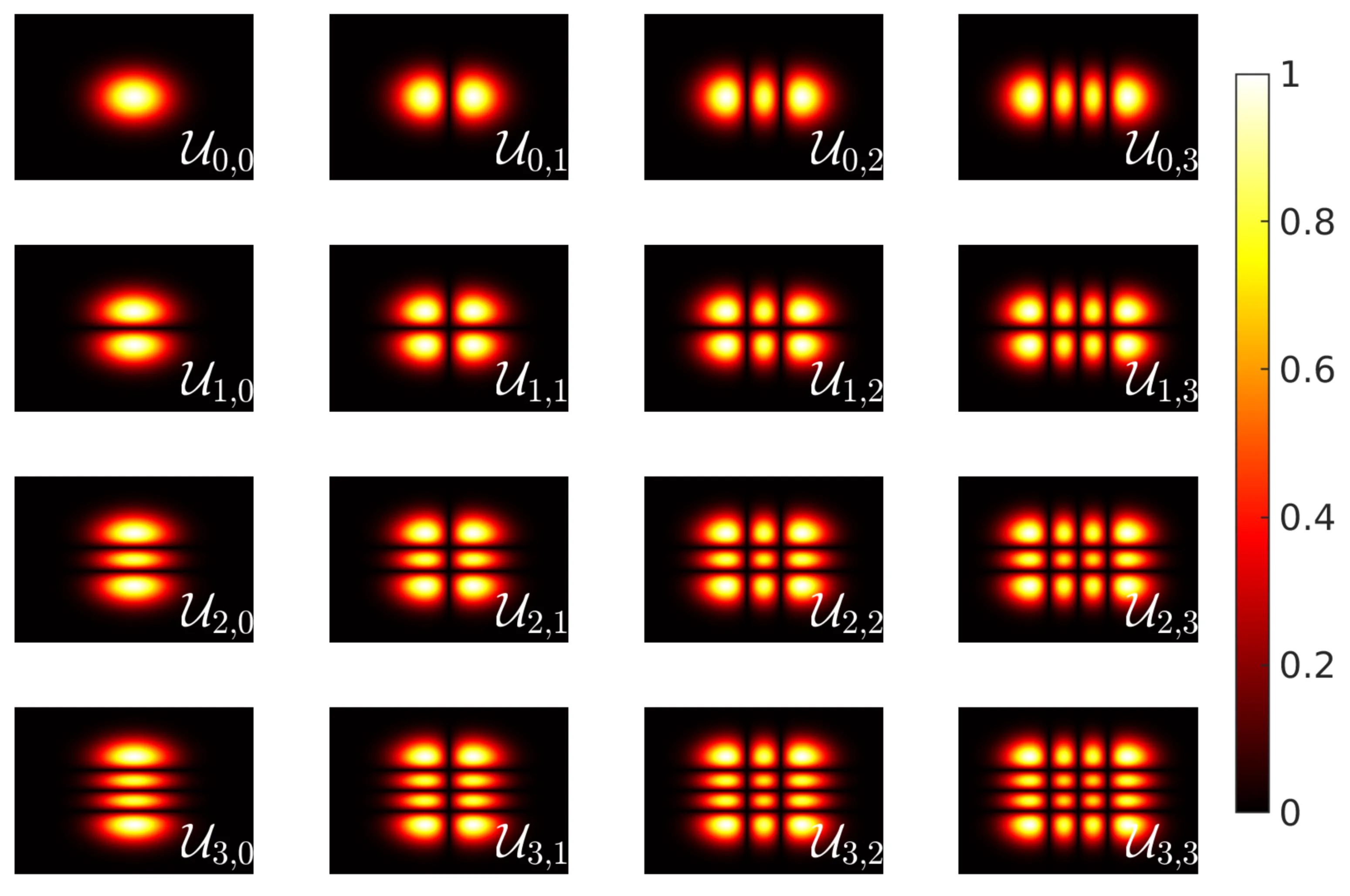
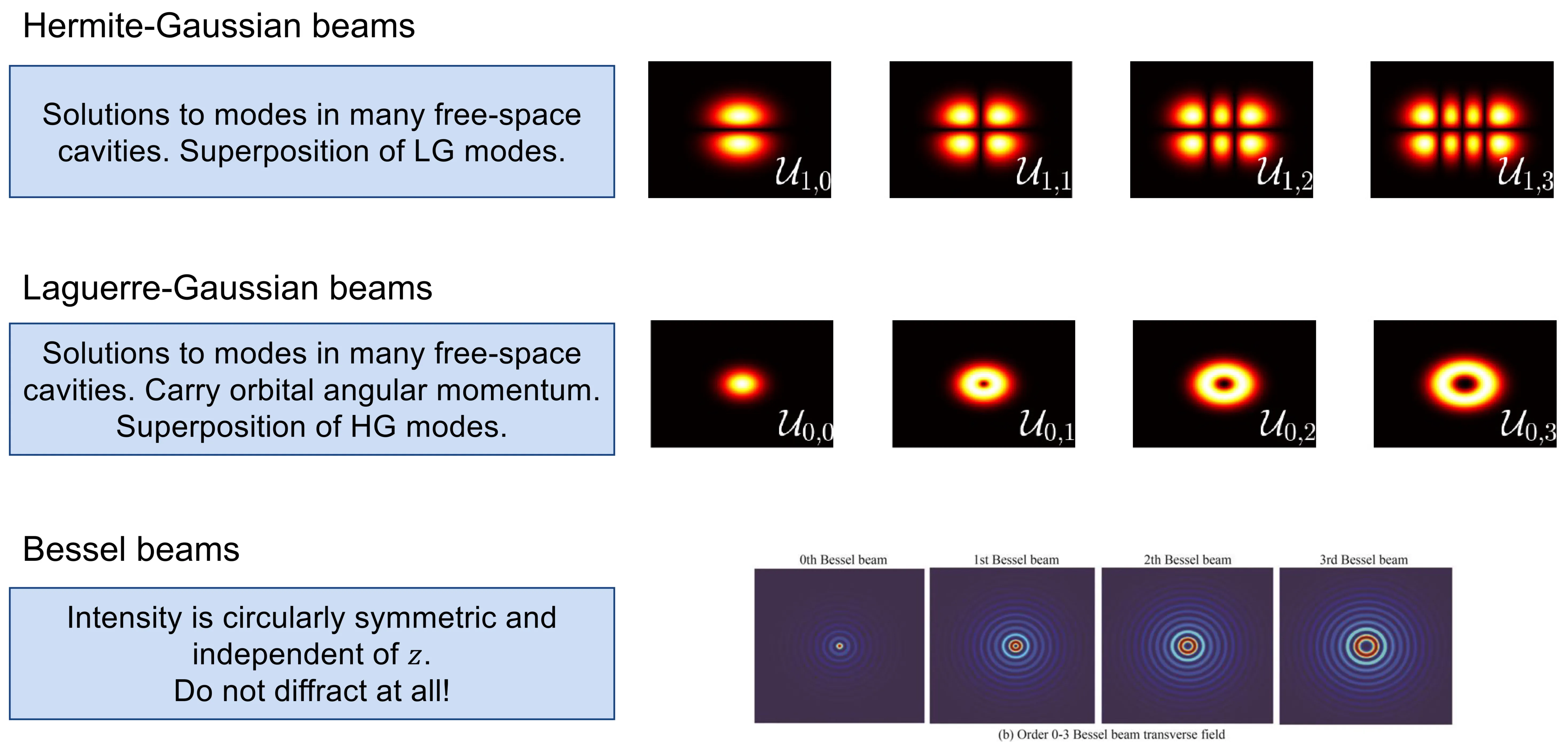
Low-order Hermite-Gaussian beam intensity profiles at the waist ( $z = z_{w}$ ) are shown below:

Attachments/Notes/2025 Quantum Electronics/6 Beam Types/QE_script.webp|700

Higher-order solutions ( $l > 0$ or $m > 0$ ) exhibit nodes (lines of zero intensity) in the transverse plane; $l$ nodes in the $x$ -direction and $m$ nodes in the $y$ -direction. Hermite-Gaussian beams form a complete orthogonal set of solutions and are often used as a basis to describe laser beams in optical resonators, particularly those with rectangular symmetry defined by astigmatic components or apertures. In many laser applications, however, operation in the fundamental $T E M_{00}$ mode is desired to achieve the best beam quality, and contributions from higher-order modes are suppressed.

Attachments/Notes/2025 Quantum Electronics/6 Beam Types/QE_script 1.webp|700

6.4 Laguerre-Gaussian Beams

If the paraxial Helmholtz equation is solved in cylindrical coordinates $(ρ, ϕ, z)$ , another complete orthogonal set of solutions is found: the Laguerre-Gaussian beams. The complex amplitude of such a beam (mode $L G_{p, l}$ ) is:

\begin{aligned} U_{p, l} (ρ, ϕ, z) = & C_{p, l} \frac{W_{0}}{W (z)} {(\frac{\sqrt{2} ρ}{W (z)})}^{| l |} L_{p}^{| l |} (\frac{2 ρ^{2}}{W^{2} (z)}) \exp (- \frac{ρ^{2}}{W^{2} (z)}) \\ \times \exp [- i k z - i k \frac{ρ^{2}}{2 R (z)} - i l ϕ + i (2 p + | l | + 1) \arctan (\frac{z - z_{w}}{z_{R}})], \end{aligned}

where $L_{p}^{| l |} (x)$ are the generalised Laguerre polynomials, $p \geq 0$ is the radial mode index (number of radial nodes excluding the one at $ρ = \infty$ ), and $l$ is the azimuthal mode index or topological charge (an integer). The fundamental Gaussian beam is $L G_{0, 0}$ ( $p = 0, l = 0$ ).
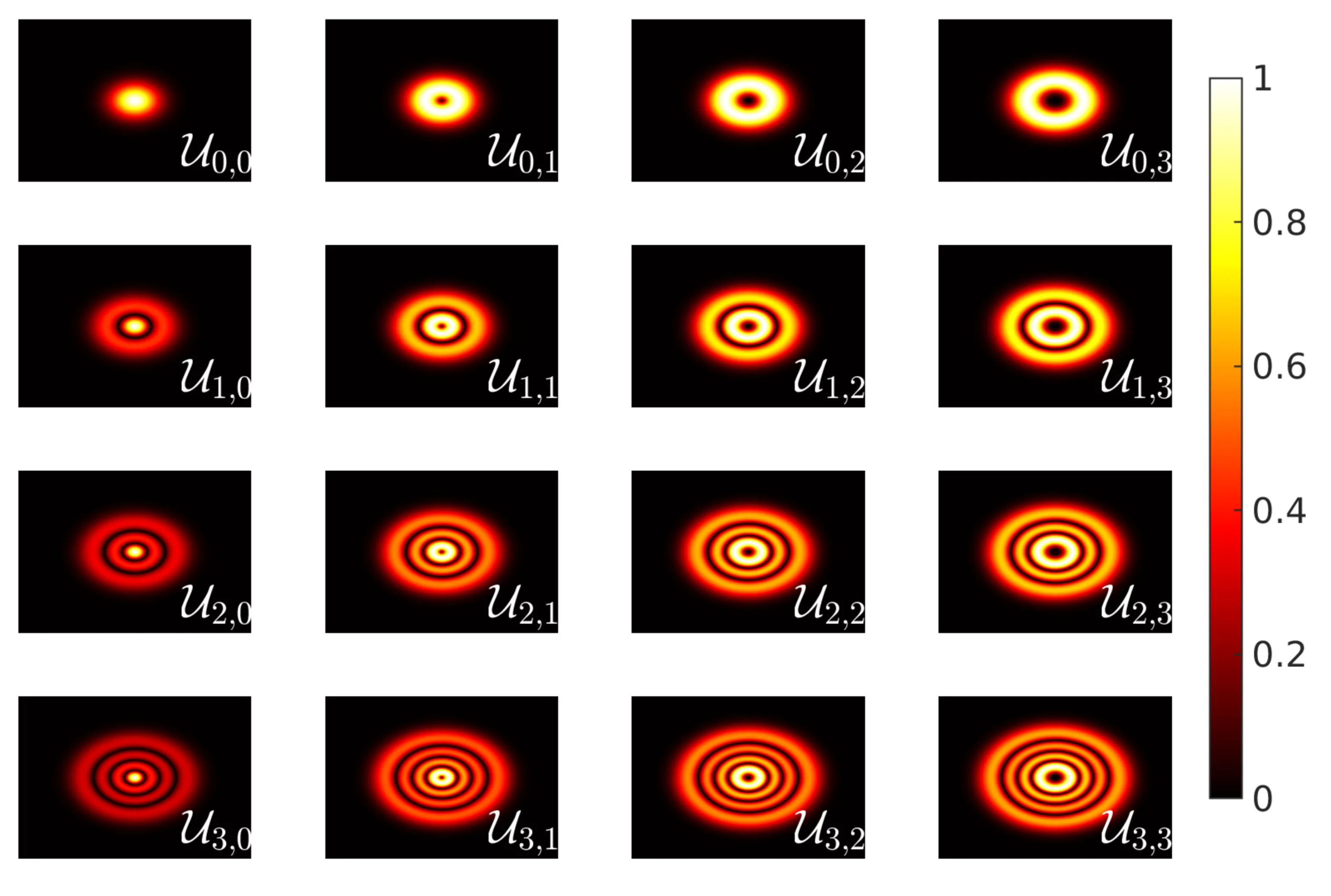
The intensity profiles of Laguerre-Gaussian beams typically exhibit cylindrical symmetry for $l = 0$ (donut shape for $p > 0, l = 0$ ) or more complex ringed structures with azimuthal phase variation $e^{- i l ϕ}$ for $l \neq 0$ . Beams with $l \neq 0$ have zero intensity on the beam axis ( $ρ = 0$ ) and possess a helical wavefront. This helical phase means these beams carry orbital angular momentum (OAM) of $l ℏ$ per photon. This OAM can impart a torque on microscopic objects, making Laguerre-Gaussian beams useful for optical tweezers, particle manipulation (rotation), and in quantum information. The following figure shows intensity profiles for some low-order Laguerre-Gaussian beams:

Attachments/Notes/2025 Quantum Electronics/6 Beam Types/QE_script 2.webp|700

The sign of $l$ determines the handedness (direction of rotation) of the helical phase front. The magnitude of $| l |$ indicates how many $2 π$ phase twists occur around the circumference.

6.5 Bessel Beams

Yet another approach to finding beam solutions involves seeking beams that are "diffraction-free" or "non-diffracting," meaning their transverse intensity profile ideally does not change upon propagation. These are distinct from Gaussian beams, which inherently diverge. An ideal Bessel beam has a field profile of the form:

U (x, y, z) = A (x, y) e^{- i k_{z} z},

where $k_{z}$ is the longitudinal wave number. Substituting this into the Helmholtz equation $\nabla^{2} U + k^{2} U = 0$ gives for the transverse amplitude $A (x, y)$ :

\nabla_{T}^{2} A (x, y) + (k^{2} - k_{z}^{2}) A (x, y) = 0 ⟹ \nabla_{T}^{2} A (x, y) + k_{T}^{2} A (x, y) = 0,

where $k_{T} = \sqrt{k^{2} - k_{z}^{2}}$ is the transverse wave number. In polar coordinates $(ρ, ϕ)$ , solutions are of the form:

A (ρ, ϕ) = A_{m} J_{m} (k_{T} ρ) e^{i m ϕ} .

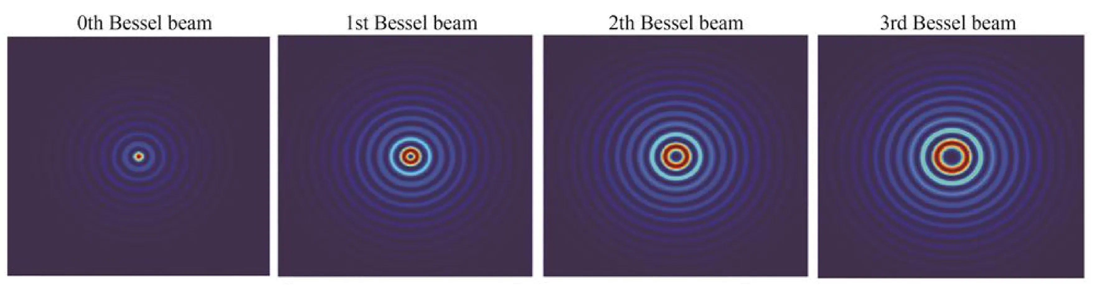
Here, $J_{m} (x)$ are Bessel functions of the first kind of order $m$ . For the fundamental Bessel beam ( $m = 0$ ), $A (ρ) = A_{0} J_{0} (k_{T} ρ)$ , which is real (for real $A_{0}$ ) and cylindrically symmetric. The wavefronts $e^{- i k_{z} z}$ are planar. The transverse intensity profile $| J_{0} (k_{T} ρ) |^{2}$ consists of a central bright spot surrounded by concentric rings, and this profile ideally propagates indefinitely without spreading:

Attachments/Notes/2025 Quantum Electronics/6 Beam Types/QE_script 3.webp|700

Bessel beams are exact solutions to the full Helmholtz equation (not just the paraxial one, though they can also be paraxial if $k_{T} ≪ k_{z}$ ). This non-diffracting property is remarkable. Such beams are also, for instance, solutions to the wave equation in an optical fibre (as guided modes).

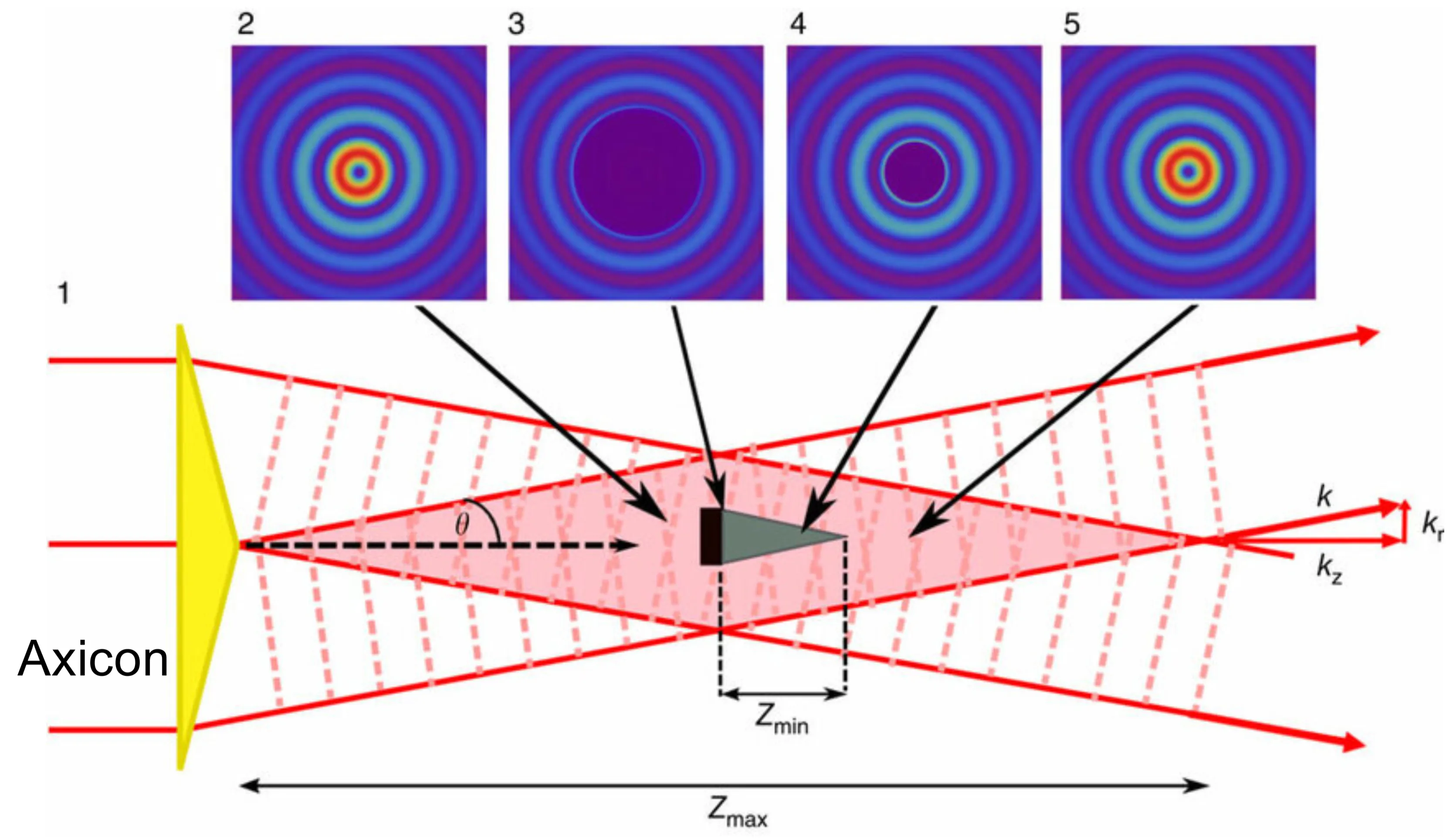
However, an ideal Bessel beam (extending infinitely in the transverse plane) carries infinite power, which is not physically realisable. In practice, Bessel beams can only be approximated over a finite transverse region and for a finite propagation distance. They can be generated experimentally using, for instance, an axicon lens, a conical lens that transforms an incident plane wave or Gaussian beam into an approximation of a Bessel beam over a certain range, or by using spatial light modulators (SLMs) to shape the wavefront.

Attachments/Notes/2025 Quantum Electronics/6 Beam Types/03_Beams_and_resonators 3.webp|700

6.6 Summary

To summarise the transverse intensity profiles of these three (excluding the fundamental Gaussian beam, which is $T E M_{00}$ or $L G_{00}$ ) beam types:

Attachments/Notes/2025 Quantum Electronics/6 Beam Types/03_Beams_and_resonators 2.webp|700