Jump back to chapter selection.

Table of Contents

5.1 Plane Waves and the Helmholtz Equation
5.2 Paraxial Approximation
5.3 Fresnel Approximation
5.4 The Fraunhofer Limit: Far Field
5.5 Diffraction Patterns -  Amplitude Modulation
5.6 Fourier Optics with a Lens
5.7 Holography
5.8 Paraxial Ray Optics

5 Fourier Optics

In this chapter, we will use a plane wave expansion of a monochromatic field to study light propagation through an optical system. The simplest of these systems is free space. It will soon become clear why this chapter is specifically titled 'Fourier' Optics.

5.1 Plane Waves and the Helmholtz Equation

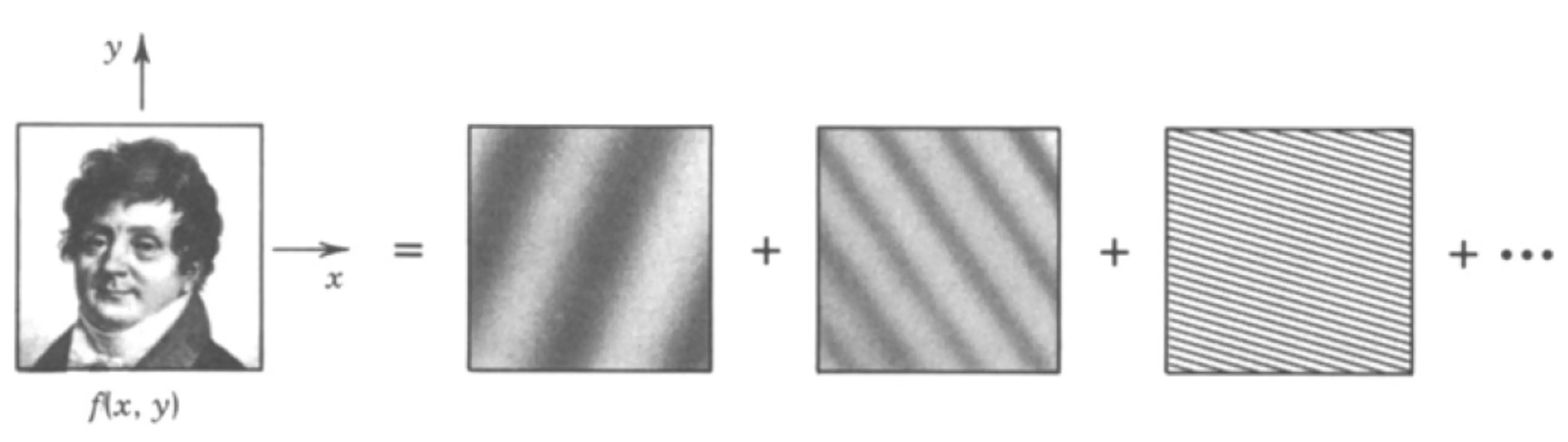
As we have seen previously, an arbitrary function may often be constructed from a sum or integral of harmonic functions (plane waves) of different frequencies and complex amplitudes. This principle extends to multiple dimensions: an arbitrary spatial function $f(x,y)$, representing for instance a field distribution in a plane, may be constructed as a superposition of harmonic functions with different spatial frequencies ($k_x,k_y$) and complex amplitudes:

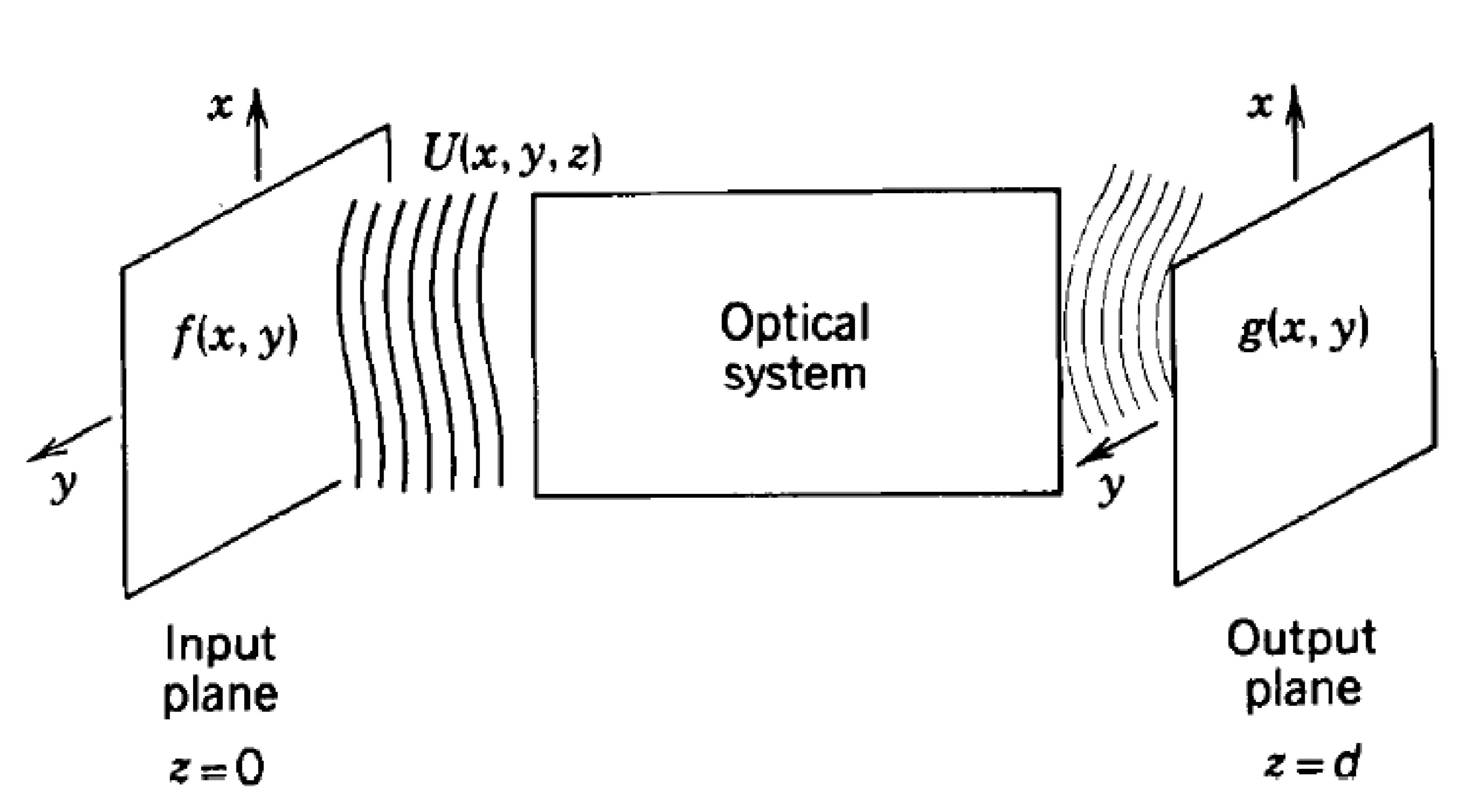
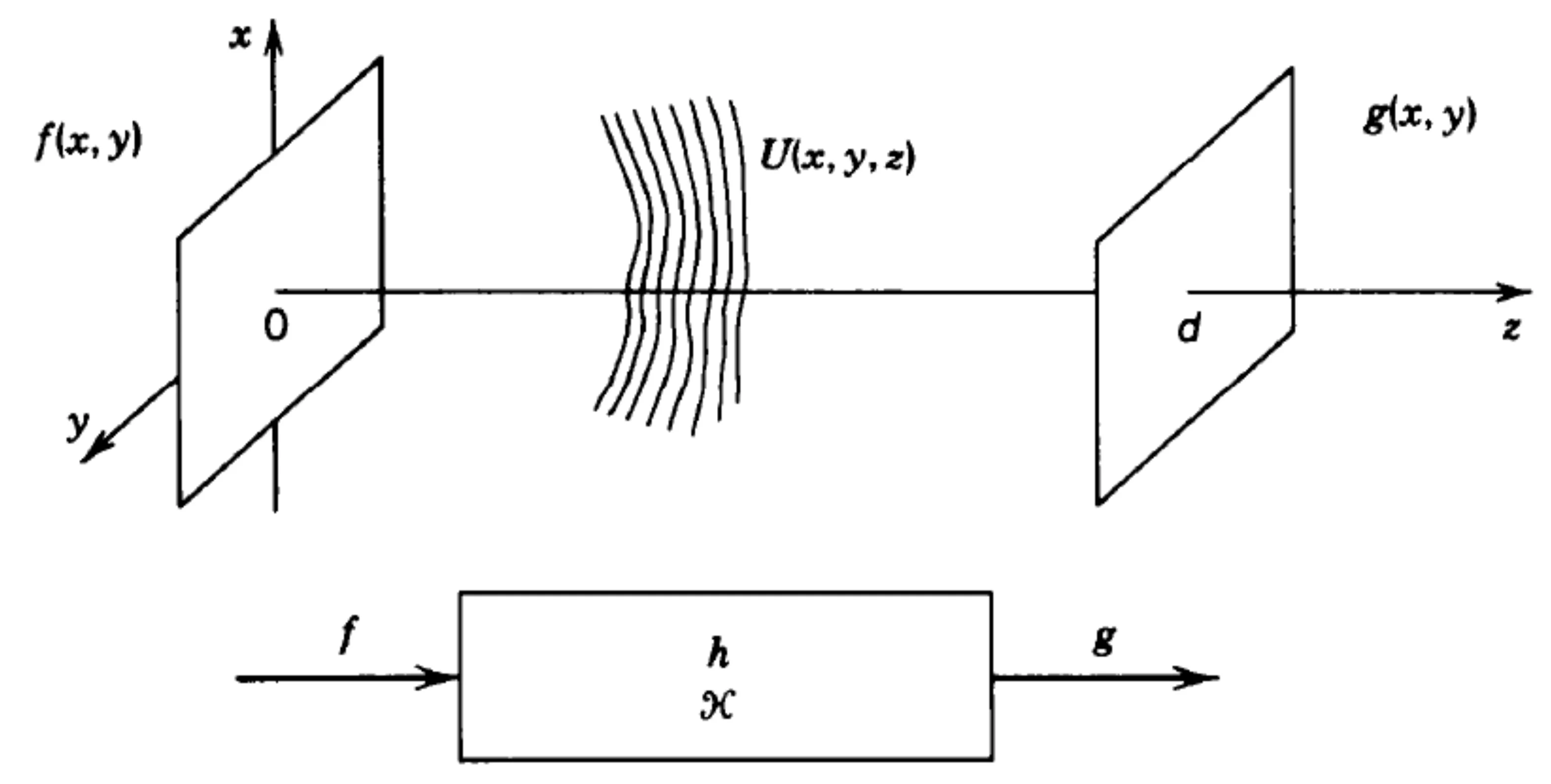
In the figures above, we describe the optical wave with a scalar function $U(x,y,z)$, which could represent, for example, one Cartesian component of the electric field. The problem at hand is the following: We consider the transmission of an optical wave $U(x,y,z)$ through an optical system, which is assumed to be linear. The input field is defined in an initial plane, say $U(x,y,0)$, and we wish to find the field in an output plane, $U(x,y,z_d)$, after propagation through a distance $z_d$:

As described in more detail here, a linear system is characterised by its impulse response or, equivalently, by its response to a harmonic function (its transfer function).

We begin the discussion of Fourier optics by recalling the wave equation for the electric field in a source-free, homogeneous, linear, isotropic, and non-dispersive medium (as derived in Chapter 1):

For a monochromatic wave, we may write the electric field as $\mathbf{E}(\mathbf{r},t)=\mathfrak{Re}[{\hat{\mathbf{e}}}_{0}U(\mathbf{r})e^{i\omega t}]$, where ${\hat{\mathbf{e}}}_0$ is a constant unit vector indicating polarisation, $U(\mathbf{r})$ is a complex scalar function of space representing the complex amplitude (magnitude and phase) of the field component, and $e^{i\omega t}$ is the time-harmonic factor (using the physics convention, where often $e^{-i\omega t}$ is used for time evolution in engineering). Substituting this into the wave equation yields the Helmholtz equation for the spatial part $U(\mathbf{r})$:

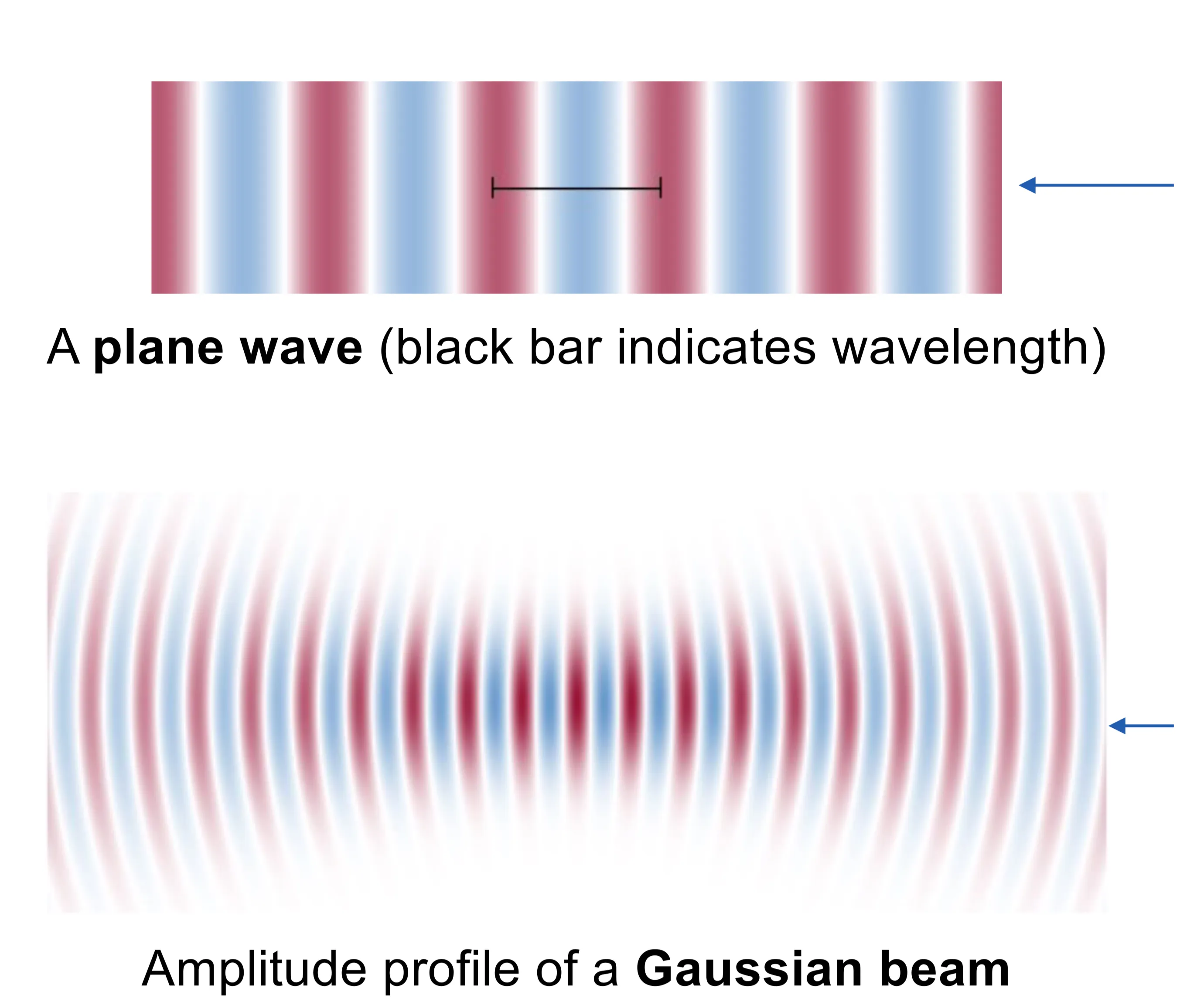
with $k=n\omega /c$ being the wave number in the medium. The time-averaged intensity is then obtained as $I(\mathbf{r})=\frac{1}{2Z}|U(\mathbf{r}){|}^2$, where $Z$ is the impedance of the medium. For the previously discussed monochromatic plane waves, $|U(\mathbf{r})|$ is constant (independent of $\mathbf{r}$). However, the Helmholtz equation also describes beams where the intensity is not uniform in space, such as Gaussian beams.
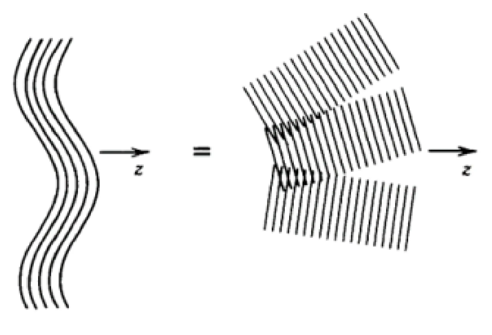
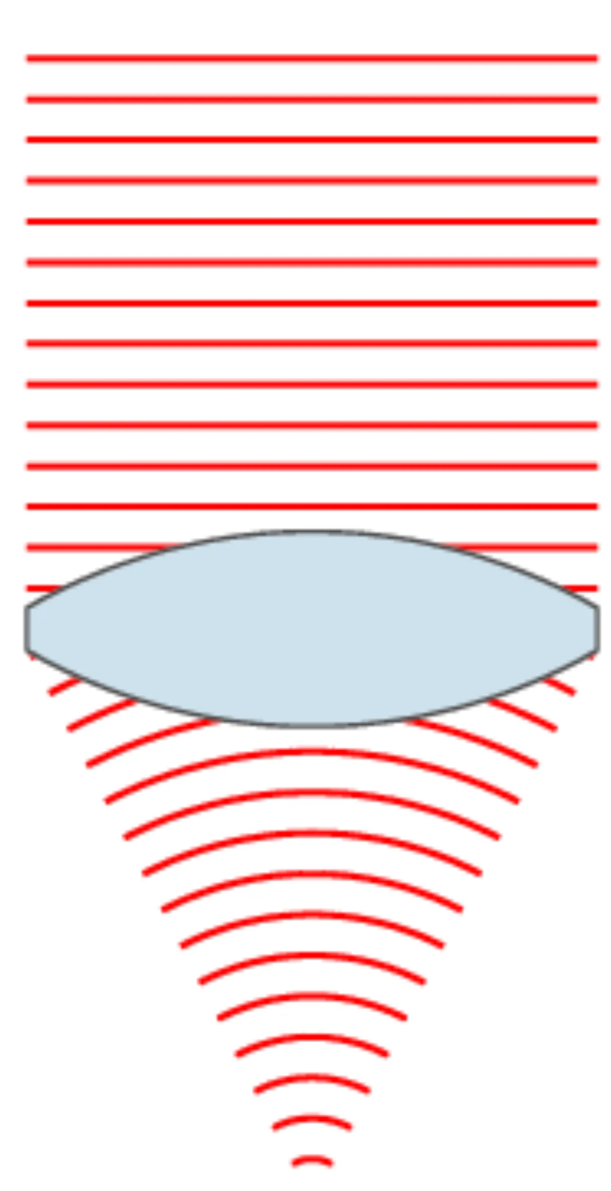
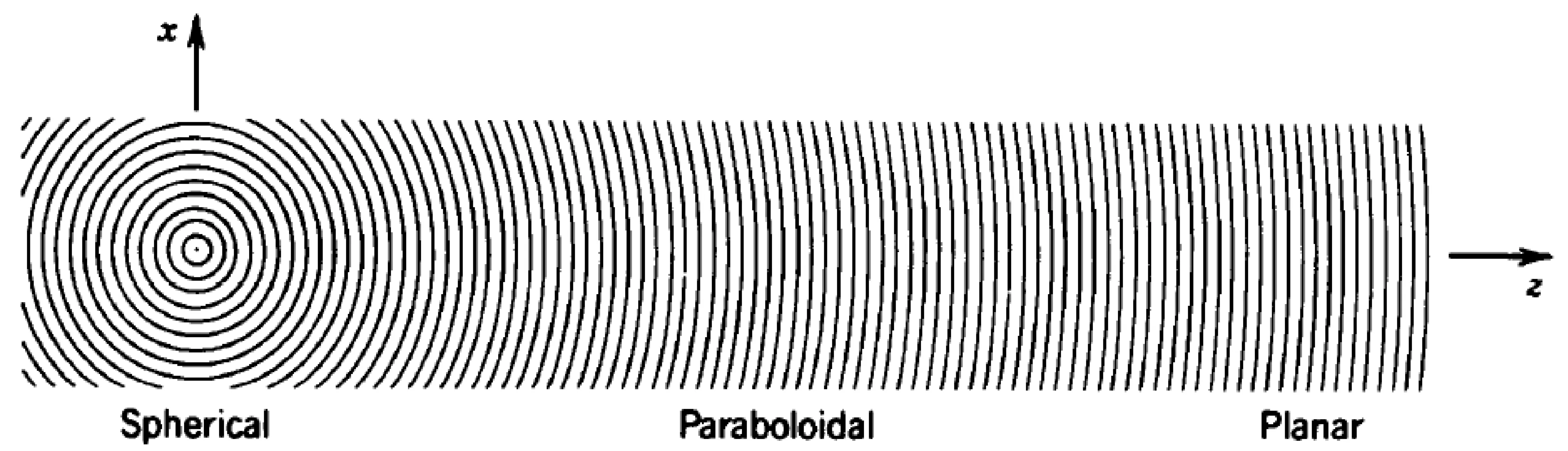
For such waves, we define the notion of a wavefront: a wavefront is a surface of constant phase. That is, if $\varphi (\mathbf{r})=\arg [U(\mathbf{r})]$, a wavefront is a 2-D surface on which $\varphi (\mathbf{r})$ is constant (modulo $2\pi$).

We can see that the wavefronts change curvature upon propagation in a Gaussian beam. For a plane wave, the wavefronts are planes. As we may expect, these wavefronts bend when passing through optical components, such as lenses:

5.2 Paraxial Approximation

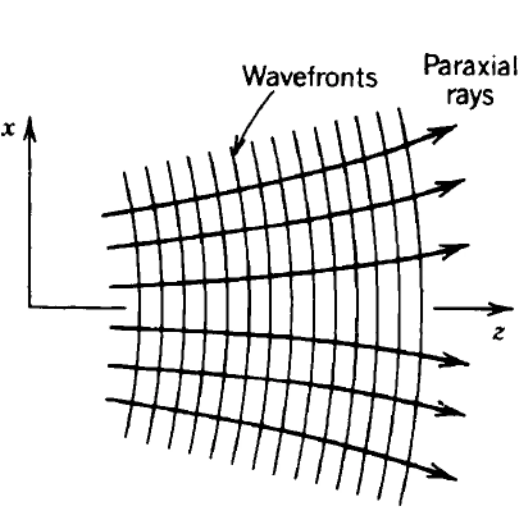
In the paraxial approximation, we assume that the light rays (normals to the wavefronts) form only small angles with the principal axis of propagation (conventionally the $z$-axis). Therefore, the transverse components of the wavevector, $k_x$ and $k_y$, which encode deviations from propagation straight along the $z$-axis, are assumed to be much smaller than the total wave number $k$. This approximation is valid for beams with small divergence angles, as is often the case for the output of a laser.

For a field $U(x,y,z)$ at a fixed plane $z$, we can define its two-dimensional spatial Fourier transform $V(k_x,k_y,z)$ with respect to the transverse coordinates $x$ and $y$:

The inverse transformation is:

Each component $(k_x,k_y)$ in this expansion corresponds to a plane wave whose wavevector is $\mathbf{k}=k_x\hat{\mathbf{x}}+k_y\hat{\mathbf{y}}+k_z\hat{\mathbf{z}}$, where $k_z$ is determined by the Helmholtz equation: $k_x^2+k_y^2+k_z^2=k^2=(n\omega /c{)}^2$. Thus, $k_z=\sqrt{k^2-k_x^2-k_y^2}$.
The paraxial approximation can be formally stated as $k_x^2+k_y^2\ll k^2$.

Applying the 2D Fourier transform (with respect to $x,y$) to the Helmholtz equation ${\mathrm{\nabla }}^{2}U+k^{2}U=0$, where ${\mathrm{\nabla }}^2={\partial }^2/\partial x^2+{\partial }^2/\partial y^2+{\partial }^2/\partial z^2$:
${\mathcal{F}}_{xy}\{{\partial }^{2}U/\partial x^2\}=(-i{k}_x{)}^{2}V=-k_x^{2}V$. Similarly for $y$.
So, we obtain an ordinary differential equation for $V(k_x,k_y,z)$ with respect to $z$:

Recognising $k_z^2=k^2-k_x^2-k_y^2$, this is $\frac{{\partial }^{2}V}{\partial z^2}+k_z^{2}V=0$.
The solution for forward propagation in $z$ is:

We define the transfer function of free space propagation over distance $z$ as:

Thus, $V(k_x,k_y,z)=V(k_x,k_y,0)H(k_x,k_y,z)$. Note that $k_z$ depends on $k_x$ and $k_y$, so $H$ is not dependent on an independent $k_z$ variable but rather on $k_x,k_y,k,$ and $z$. This approach is valid for propagation in any homogeneous isotropic medium.
Knowing $U(x,y,0)$ in an initial plane allows us to find its profile $U(x,y,z)$ in any other plane at a distance $z$:

The procedure is:

1. Calculate the 2D spatial Fourier transform $V(k_x,k_y,0)$ of the input field $U(x,y,0)$.
2. Multiply $V(k_x,k_y,0)$ by the transfer function $H(k_x,k_y,z)$ to obtain $V(k_x,k_y,z)$.
3. Apply the inverse 2D spatial Fourier transform to $V(k_x,k_y,z)$ to obtain $U(x,y,z)$.

It is important to remember that we are working with linear systems: harmonic components (spatial frequencies $k_x,k_y$) are not created or destroyed during propagation in a linear homogeneous medium; only their relative phases are modified by $H(k_x,k_y,z)$.

5.3 Fresnel Approximation

In the expression for the transfer function $H(k_x,k_y,z)$, the term $k_z=\sqrt{k^2-k_x^2-k_y^2}$ makes analytical inverse Fourier transformation difficult. In the paraxial approximation ($k_x^2+k_y^2\ll k^2$), the angles ${\theta }_x\approx k_x/k$ and ${\theta }_y\approx k_y/k$ of the constituent plane waves with respect to the $z$-axis are small. We can then expand the phase of the transfer function, $k_{z}z$:

Using the Taylor expansion $\sqrt{1-u}\approx 1-u/2-u^2/8-\dots$ for small $u$:

The Fresnel approximation (or paraxial wave equation approximation) consists of keeping terms only up to the first order in $u=(k_x^2+k_y^2)/k^2$ within the square root, which means keeping terms quadratic in $k_x,k_y$:

This approximates the spherical wavefront segment of each plane wave component with a parabolic one. The simplified transfer function becomes:

We can write $H_0=e^{ikz}$, which is the phase accumulated by a plane wave propagating along $z$.
The Fresnel approximation implies that we are observing the field at a distance $z$ that is large compared to the transverse extent of the source/aperture, but not so large that the wavefronts become essentially planar over the observation region (which leads to Fraunhofer diffraction).

Considering the source of the wave to be spherical, the Fresnel approximation approximates these spherical wavefronts with parabolas:

The validity of the Fresnel approximation requires that the next term in the Taylor expansion of the phase, $kz\frac{1}{8}{\left(\frac{k_x^2+k_y^2}{k^2}\right)}^2$, must be much less than $\pi$. This is a stricter condition than just $k_x^2+k_y^2\ll k^2$. It can be related to the Fresnel number $N_F=a^2/(\lambda z),$ where $a$ is a characteristic transverse dimension (of aperture or beam).

Next, we find the impulse response $h(x,y,z)$ for Fresnel propagation, which is the field at $(x,y,z)$ due to a point source $U(x^{\prime },y^{\prime },0)=\delta (x^{\prime })\delta (y^{\prime })$.

1. The 2D Fourier transform of $U(x^{\prime },y^{\prime },0)=\delta (x^{\prime })\delta (y^{\prime })$ is $V(k_x,k_y,0)=\iint \delta (x^{\prime })\delta (y^{\prime })e^{i(k_x{x}^{\prime }+k_y{y}^{\prime })}d{x}^{\prime }d{y}^{\prime }=1$.
2. Therefore, $V(k_x,k_y,z)=1\cdot H(k_x,k_y,z)=e^{ikz}{e}^{-iz\frac{k_x^2+k_y^2}{2k}}$.
3. We take the inverse Fourier transform:$$h(x,y,z)=U(x,y,z)=\frac{e^{ikz}}{(2\pi {)}^2}\iint e^{-iz\frac{k_x^2+k_y^2}{2k}}{e}^{-i(k_{x}x+k_{y}y)}d{k}_{x}d{k}_y.$$

We find that the impulse response function $h(x,y,z)$ is given by:

This impulse response is useful because for a linear system, the output $U(x,y,z)$ for an arbitrary input $U(x^{\prime },y^{\prime },0)$ is given by the convolution:

Substituting $h(x-x^{\prime },y-y^{\prime },z)$:

This is the Fresnel diffraction integral.

The general steps to find the electric field $U(x,y,z)$ for a given input $U(x,y,0)$ are:

1. Find the 2D spatial Fourier transform $V(k_x,k_y,0)$ of $U(x,y,0)$.
2. Multiply by the appropriate transfer function $H(k_x,k_y,z)$ to obtain $V(k_x,k_y,z)$.
3. Apply the inverse 2D spatial Fourier transform to $V(k_x,k_y,z)$ to obtain $U(x,y,z)$.

5.4 The Fraunhofer Limit: Far Field

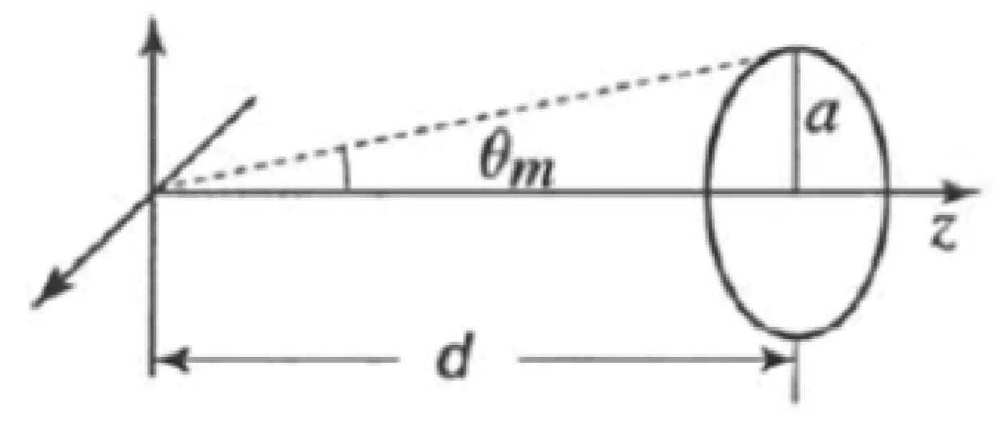
The Fraunhofer approximation, or far-field diffraction, is a limit of the Fresnel approximation valid at sufficiently large distances $z$ from an aperture or object of characteristic transverse size $D_{obj}$. It requires the Fresnel conditions to be met, plus an even stronger condition.

The condition for Fraunhofer diffraction is often expressed using the Fresnel number $N_F=D_{obj}^2/(\lambda z)$. The Fraunhofer regime applies when $z\gg D_{obj}^2/\lambda$, which means $N_F\ll 1$.
If $D_{obs}$ is the size of the observation region (detector), then we also typically require $z\gg D_{obs}^2/\lambda$.

The crucial simplification in the Fraunhofer limit arises from approximating the quadratic phase term in the Fresnel integral $e^{i\frac{k}{2z}[{(x-x^{\prime })}^2+{(y-y^{\prime })}^2]}$.
We expand $(x-x^{\prime }{)}^2=x^2-2x{x}^{\prime }+x^{\prime 2}$. The term $e^{i\frac{k}{2z}(x^{\prime 2}+y^{\prime 2})}$ is kept under the integral. The term $e^{i\frac{k}{2z}(x^2+y^2)}$ is taken outside. The Fraunhofer condition allows $k(x^{\prime 2}+y^{\prime 2}{)}_{max}/(2z)\ll \pi$.
The field $U(x,y,z)$ in the Fraunhofer regime becomes:

Recognising $k_x=kx/z=2\pi x/(\lambda z)$ and $k_y=ky/z=2\pi y/(\lambda z)$ as spatial frequencies (proportional to observation angles ${\theta }_x\approx x/z,{\theta }_y\approx y/z$), the integral is the 2D Fourier transform of the input field $U(x^{\prime },y^{\prime },0)$ evaluated at these spatial frequencies:

The Fraunhofer approximation essentially states that in the far field, the observed complex amplitude is proportional to the Fourier transform of the aperture distribution, multiplied by a phase factor. All plane wave components effectively interfere constructively only along specific directions corresponding to their $(k_x,k_y)$ values, mapping spatial frequencies in the object plane to positions in the observation plane.

5.5 Diffraction Patterns - Amplitude Modulation

When an optical wave passes through an aperture or is otherwise spatially modulated in amplitude and/or phase, and then propagates some distance in free space, the resulting intensity distribution is called a diffraction pattern. From the discussion above, it should be clear that simply expecting the intensity pattern to be a geometric shadow of the aperture is an oversimplification, valid only in the limit of ray optics where the wave nature of light is ignored.
Consider an aperture described by an aperture function $p(x,y)$ in the input plane $z=0$:

If an incident wave $U_{\text{inc}}(x,y)$ illuminates this aperture, the field immediately after the aperture is $U(x,y,0)=U_{\text{inc}}(x,y)p(x,y)$. We now know, in principle, how to obtain the field $U(x,y,z)$ at some distance $z$.

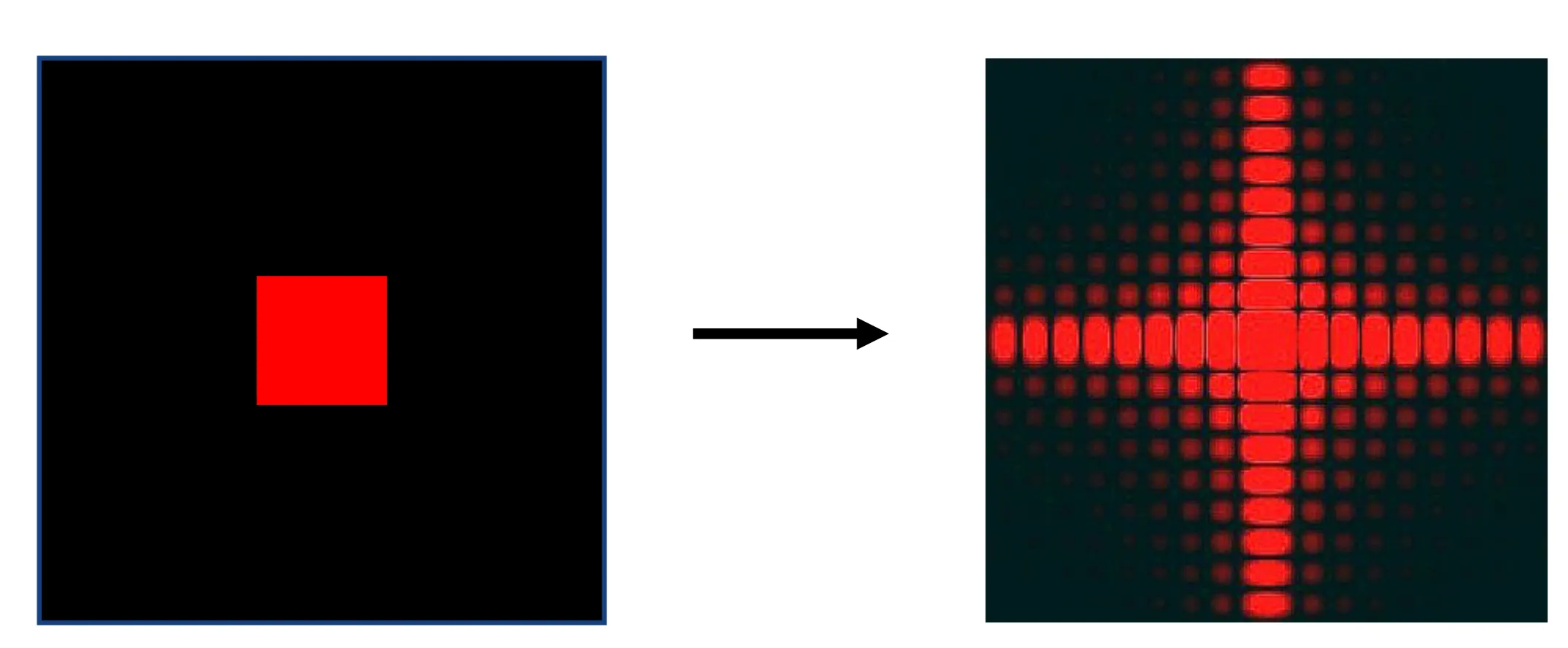
5.5.1 Rectangular Aperture

Consider a rectangular aperture of width $D_x$ and height $D_y$, centered at the origin. Assume it is illuminated by a normally incident plane wave of constant amplitude $E_{in}$ (so $U(x,y,0)=E_{in}$ inside the aperture and $0$ outside). We apply the Fraunhofer approximation to find the far-field pattern at a distance $d.$
The 2D Fourier transform $V(k_x,k_y)$ of $U(x,y,0)$ is:

where $\mathrm{sinc}(u)=\sin (\pi u)/(\pi u)$. The far-field intensity $I(x_s,y_s,d)\sim |V(k_x=k{x}_s/d,k_y=k{y}_s/d){|}^2$. If $I_0$ is related to $E_{in}^2$:

Here $I_{\text{peak}}$ is the intensity at the centre of the pattern. Then, we arrive at:

This result is expected, as the Fourier transform of a rectangular function (top-hat) is a sinc function. The intensity pattern is shown next:

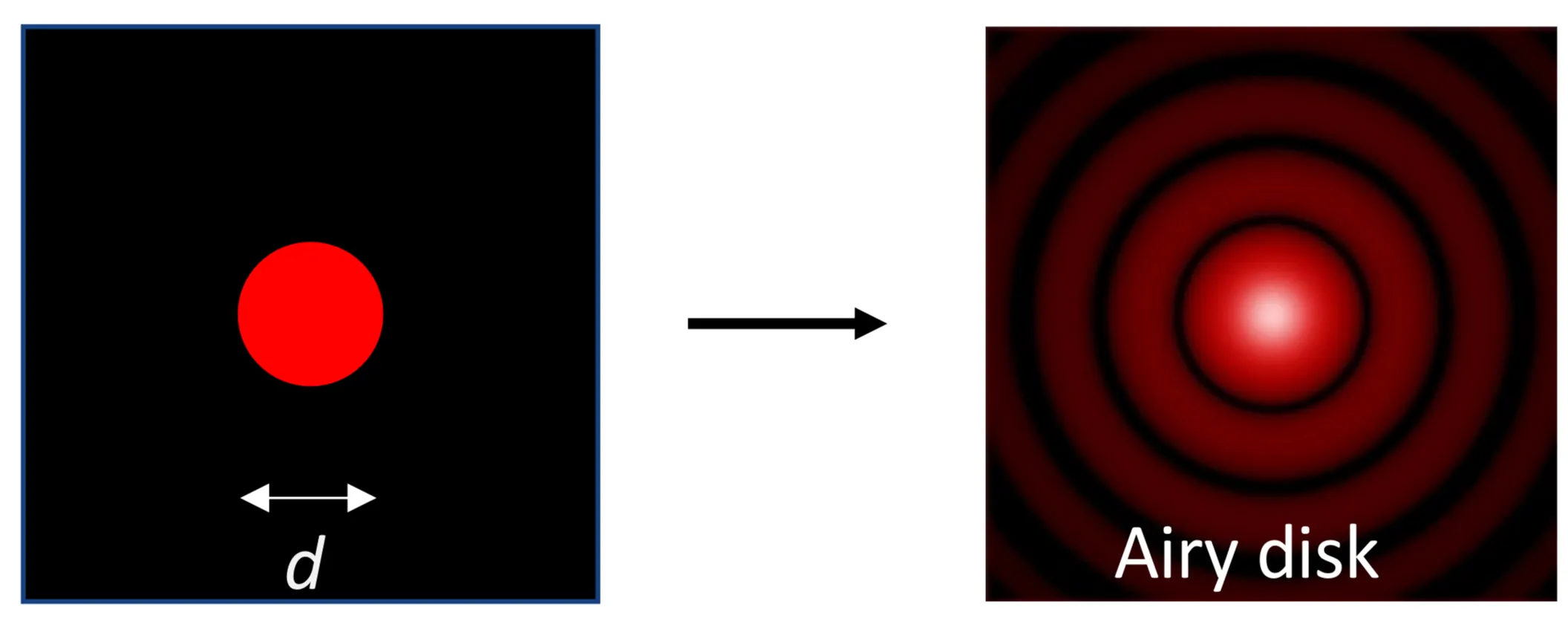
5.5.2 Circular Aperture

Consider a circular aperture of diameter $D$. The 2D Fourier transform of a circular aperture (circ function) is related to a Bessel function of the first kind, $J_1$:

where $k_{\rho }=\sqrt{k_x^2+k_y^2}$. The far-field intensity pattern at radius ${\rho }_s=\sqrt{x_s^2+y_s^2}$ on the screen is:

This is the characteristic Airy disk pattern shown in the next figure.

5.6 Fourier Optics with a Lens

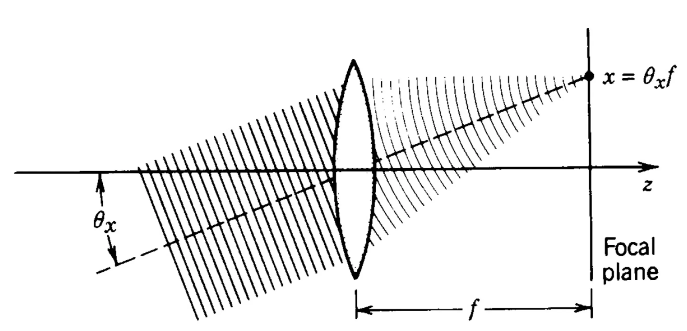
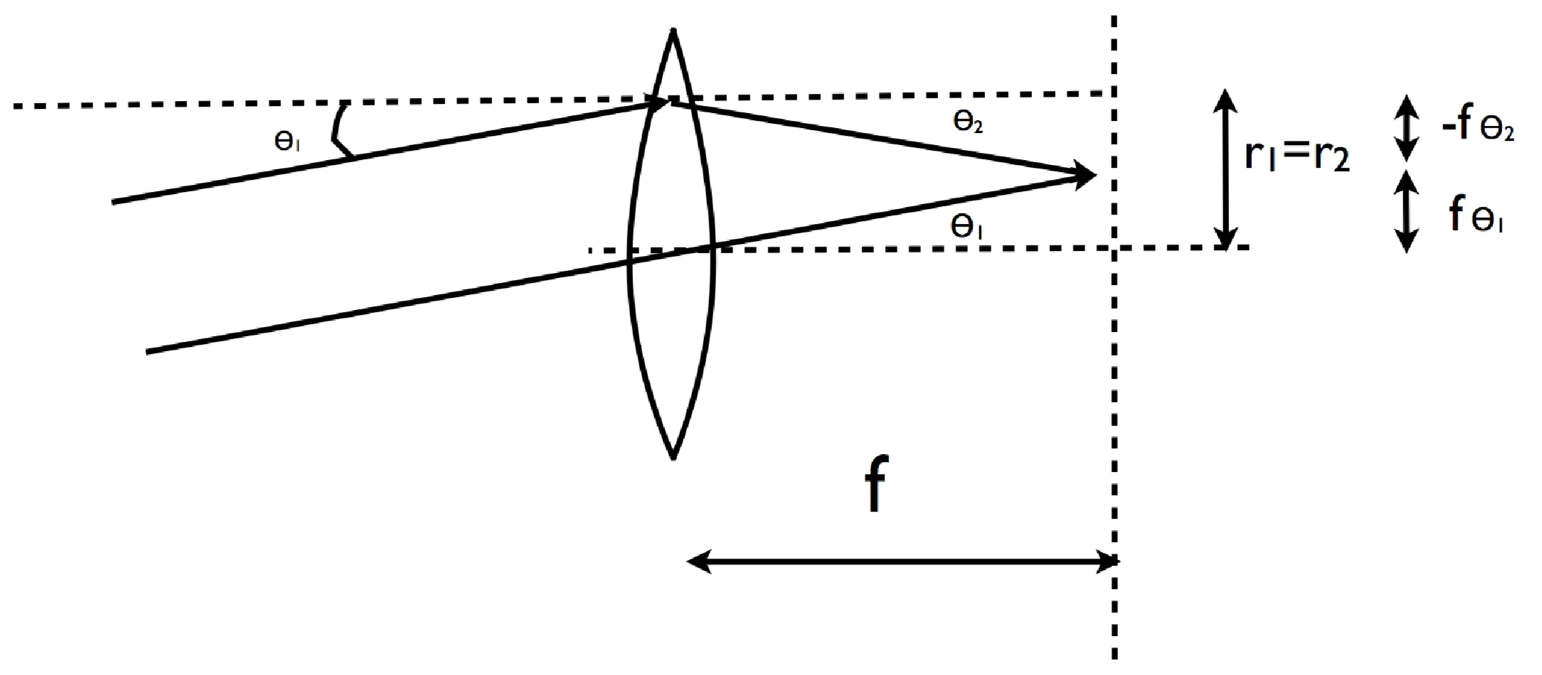
A thin lens introduces a quadratic phase transformation to an incident wavefront. For a lens with focal length $f$, its phase transfer function is $t_L(x,y)=e^{-i\frac{k}{2f}(x^2+y^2)}$ (for a focusing lens, assuming it's thin and located at $z=0$).
If an object $U_{in}(x_o,y_o)$ is placed at the front focal plane ($z=-f$) of a lens, the field at the back focal plane ($z=f$) $U_{BFP}(x_f,y_f)$ is proportional to the Fourier transform of $U_{in}$:

More generally, if an object $U(x_o,y_o)$ is placed immediately before a lens, the field at its back focal plane is proportional to the Fourier Transform of $U(x_o,y_o)$:

The integral is $V(k_x=k{x}_f/f,k_y=k{y}_f/f)$, where $V$ is the FT of $U(x_o,y_o,0^{-})$ with the appropriate FT kernel sign. This demonstrates the Fourier transforming property of a lens.

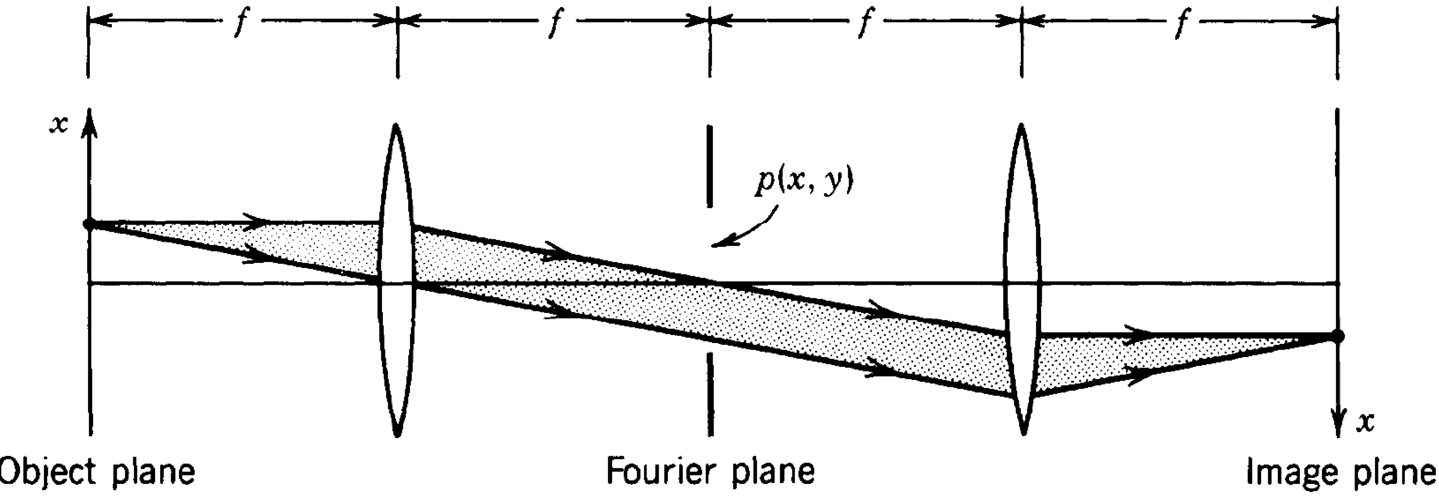
A common configuration is a 2f system, where an object is placed at distance $f$ before a lens, and the image (which is the Fourier transform) is observed at distance $f$ after the lens. If another identical lens is placed at $2f$, it performs an inverse Fourier transform, potentially forming an inverted image of the original object at $4f$ from the first object plane. This is a 4f system:

In the Fourier plane (at $2f$ from the object, between the two lenses), one can place an amplitude or phase mask $P(x_F,y_F)$ to filter out or modify specific spatial frequency components of the object. Here $x_F,y_F$ are coordinates in the Fourier plane, related to spatial frequencies $k_x,k_y$ by $k_x\approx k{x}_F/f,k_y\approx k{y}_F/f$. The transfer function of such a spatial filtering system is effectively $H(k_x,k_y)\approx P(x_F=\lambda f{k}_x/(2\pi ),y_F=\lambda f{k}_y/(2\pi ))$.
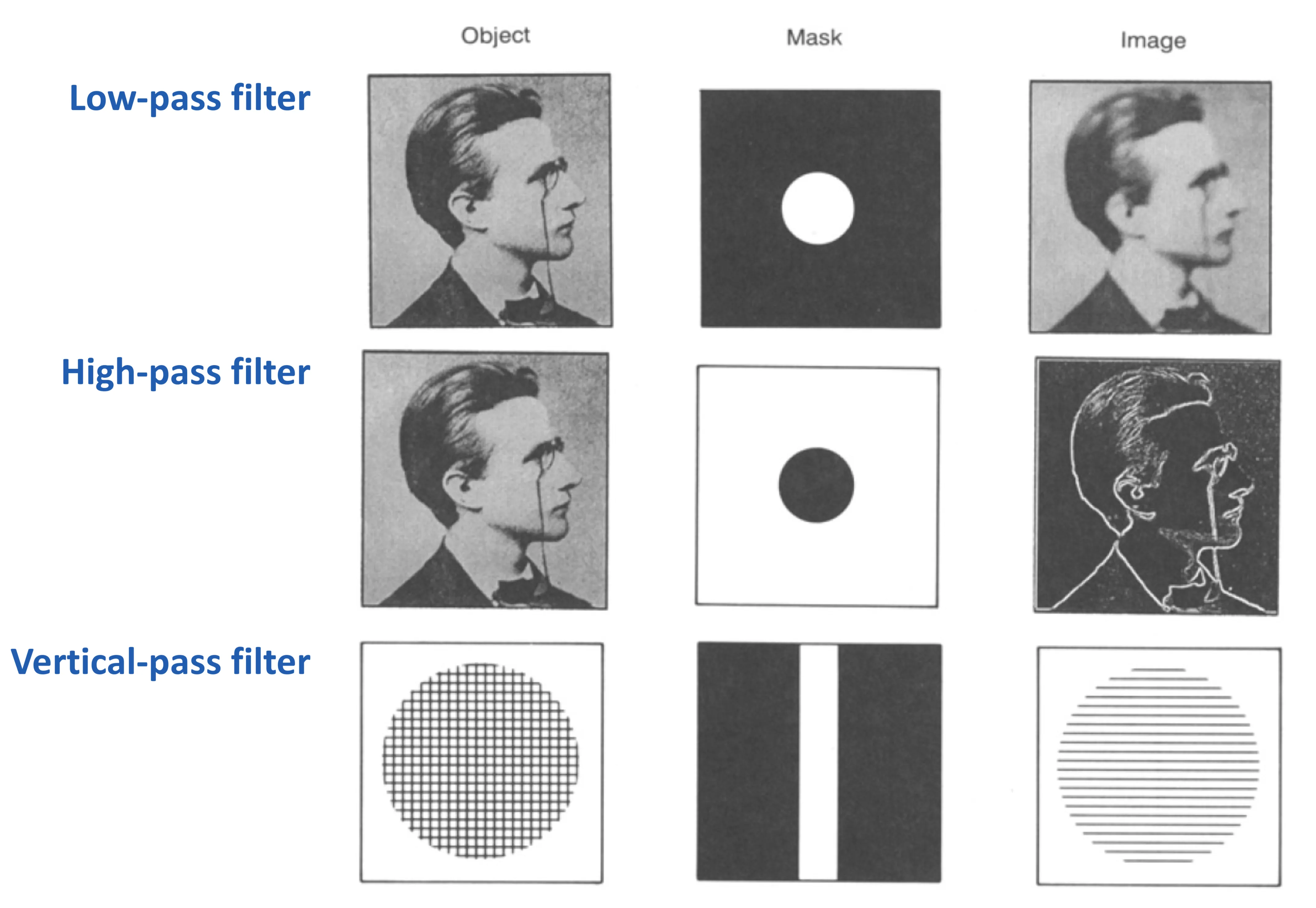
Consider the image example: A standard circular aperture in the Fourier plane acts as a low-pass filter, blurring the image by removing high spatial frequencies (sharp details). An opaque stop in the centre acts as a high-pass filter, enhancing edges and removing large-scale variations, making the man's skin appear dark while highlighting hair.

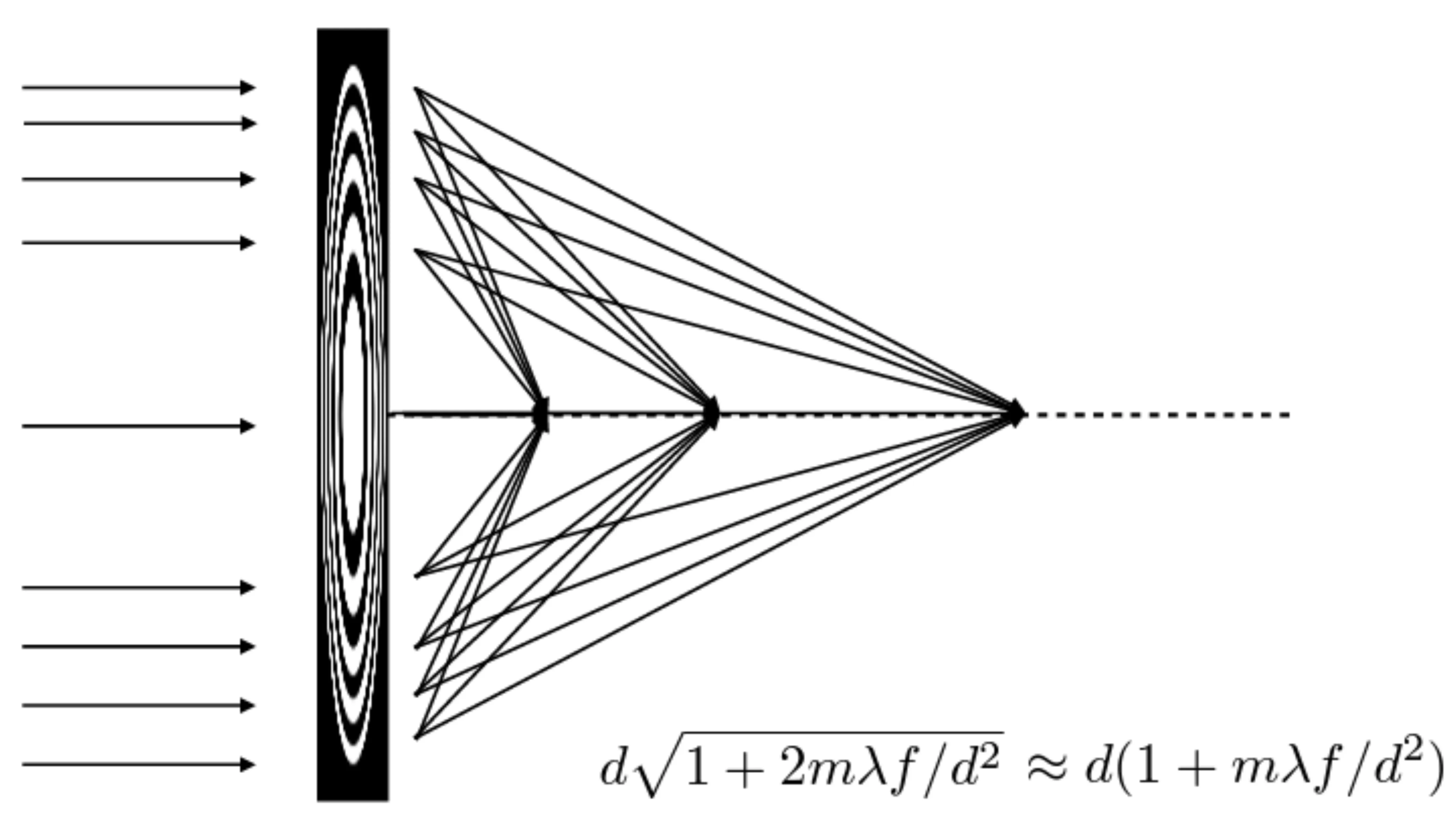
A Fresnel zone plate is another optical element that can focus light, but it operates based on diffraction rather than refraction.

Its transmission function $t(x,y)$ consists of concentric transparent and opaque zones:

for a binary zone plate designed for focal length $f$.

The spacing of these Fresnel zones is such that light diffracted from the transparent zones interferes constructively at the desired focal point. Zone plates are inherently chromatic, focusing different wavelengths to different focal points.

5.7 Holography

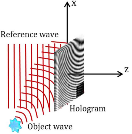
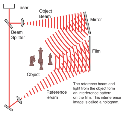
Holograms are recordings that encode the full optical wave from an object, including both its amplitude and phase information. In principle, if we could create a transparency $t(x,y)$ equal to the complex field $U(x,y,0)$ from an object, illuminating this transparency with a plane wave would reconstruct the object wave. However, optical detectors are sensitive only to intensity ($|U{|}^2$), not directly to phase. Holography overcomes this by interfering a reference wave $U_r$ with the object wave $U_o$.

(Image source)

If these two waves overlap at $z=0$, the intensity pattern recorded on a film (hologram) is:

Assuming the film's amplitude transmittance $t$ after development is proportional to $I_{\text{rec}}$:

where $I_r=|U_r{|}^2$ and $I_o=|U_o{|}^2$.
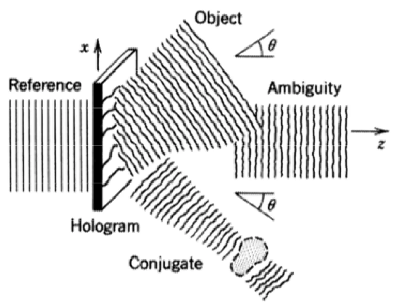
When this hologram is illuminated by the original reference wave $U_r$, the transmitted field $U_{\text{trans}}=t{U}_r$ is:

If the reference wave $U_r$ is a uniform plane wave with amplitude $A_r$ (so $I_r=A_r^2$), the terms are:

1. $A_r{I}_r$: A scaled version of the reference wave (DC term).
2. $A_r{I}_o(x,y)$: The reference wave modulated by the object intensity (distorted image).
3. $I_r{U}_o(x,y)$: A wave proportional to the original object wave $U_o$. This term reconstructs the virtual image of the object.
4. $A_r^2{U}_r{U}_o^{\ast }$: A wave related to the conjugate of the object wave. This term reconstructs the real image (often called the twin image or conjugate image).

To separate these four waves spatially, a common technique is off-axis holography, where the reference wave $U_r$ and object wave $U_o$ are incident on the recording film at a significant angle to each other:

This angular separation ensures that upon reconstruction, the four terms propagate in different directions, allowing the desired $U_o$ term to be viewed without overlap from the others.
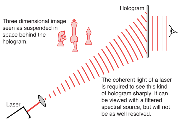
Holography generally requires light sources with high temporal and spatial coherence (such as lasers) for both recording and reconstruction. Variations like volume holography (where interference fringes are recorded throughout the depth of a thick medium) and rainbow holography (which allows viewing in white light) address some of these limitations.

Generally, we differentiate two types of hologram based on recording geometry:

• Reflection hologram: The reference and object beams approach the recording material from opposite sides. Interference fringes are typically formed in planes nearly parallel to the surface. Reconstruction is usually done by illuminating the hologram from the same side as the original reference beam was incident.
• Transmission hologram: The reference and object beams approach the film from the same side. Interference fringes are generally formed nearly perpendicular to the surface. Reconstruction is done by illuminating with the reference beam, and the reconstructed object wave is viewed by looking through the hologram.

An example of a transmission hologram setup is shown in the next figure (source).

In ordinary photography, only the intensity distribution $|U_o{|}^2$ is recorded, so all phase information is lost, and thus three-dimensional reconstruction is not possible.

5.8 Paraxial Ray Optics

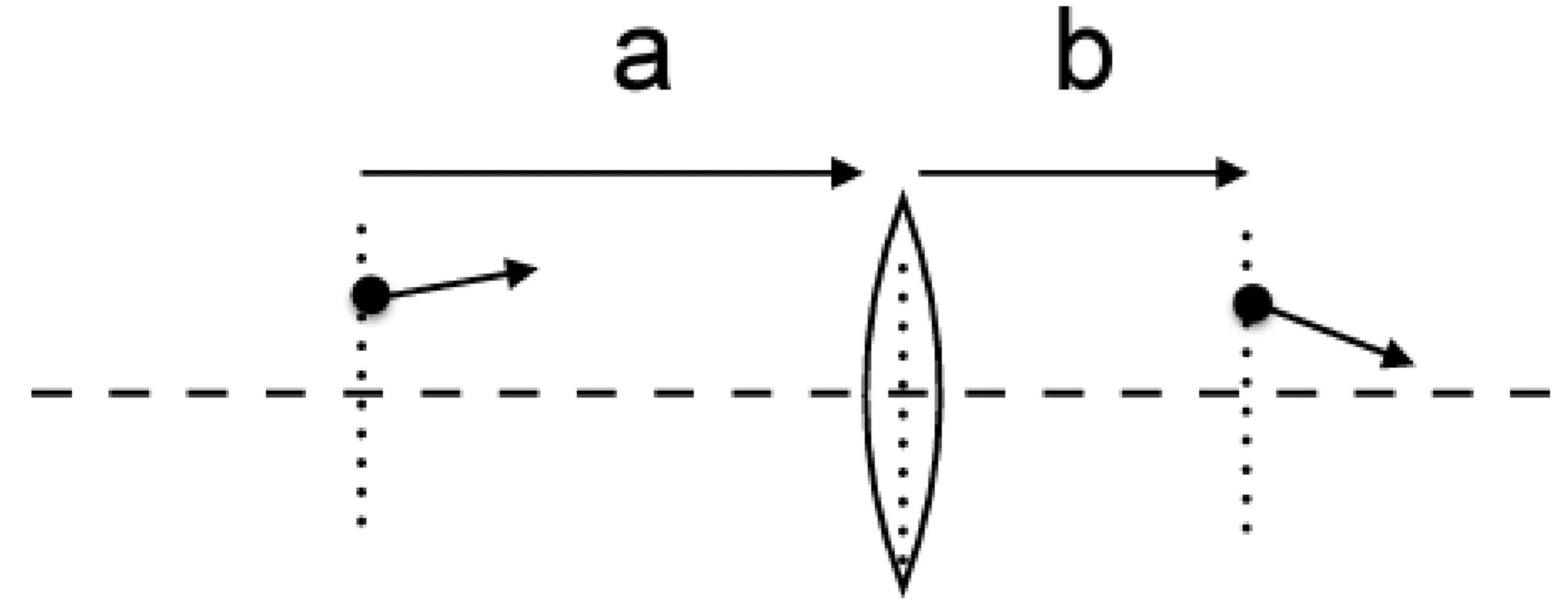
Often, for analysing simple optical systems, a full wave-optical (Fourier) treatment is not necessary, and the simpler ray approximation (geometric optics) suffices. This is especially true when effects of diffraction can be neglected, for instance, when all apertures and beam sizes are much larger than the wavelength of light. We define a ray as the local normal to a wavefront. We will work within the paraxial approximation, meaning all rays form small angles with respect to the optical axis (conventionally the $z$-axis).
A single ray at a transverse plane can be described by a 2D vector, commonly its radial distance $r$ from the axis and its angle $\theta$ with respect to that axis (or $dr/dz$). We will assume systems with cylindrical symmetry around the $z$-axis for this ray description. For example, a thin converging lens with focal length $f$ transforms an incident ray $(r_1,{\theta }_1)$ to an output ray $(r_2,{\theta }_2)$ according to:

where we have used the small angle approximation $\tan \theta \approx \sin \theta \approx \theta$.

This transformation can be expressed using a matrix, called the ABCD matrix or ray-transfer matrix, which relates the output ray vector to the input ray vector:

For the thin lens described above, the ray-transfer matrix is:

Similarly, for propagation through a homogeneous medium of length $d$, a ray $(r_1,{\theta }_1)$ becomes $(r_2,{\theta }_2)$ where $r_2=r_1+d{\theta }_1$ and ${\theta }_2={\theta }_1$. The ray-transfer matrix is:

For a planar interface between homogeneous media with refractive indices $n_1$ and $n_2$ (ray incident from $n_1$ to $n_2$ at near-normal incidence):

The effect of a spherical mirror with concave radius of curvature $R$ (light incident from left, vertex at origin, centre of curvature at $z=-R$) is equivalent to a lens with $f=R/2$:

The advantage of this matrix formalism is that the overall ray-transfer matrix for a cascade of optical elements is found by multiplying the individual matrices in the correct order (last element encountered by the ray first in the matrix product if input is on the right, or first element first if input is on the left, depending on how the output vector is written). For example, consider propagation through a medium of length $a$, followed by a lens of focal length $f$, then another propagation through length $b$:

The matrix ${\mathbf{M}}_{\text{total}}$ relating the output ray $(r^{\prime },{\theta }^{\prime })$ to the input ray $(r,\theta )$ is: