Jump back to chapter selection.

Table of Contents

4.1 Young's Double Slit Experiment
4.2 Coherence Function
4.3 Coherence Time and Coherence Length
4.4 Wiener-Khinchin Theorem
4.5 Interference
4.6 Fabry-Pérot Interferometer - Etalon
4.7 Matrix Methods for Multiple Surfaces

4 Coherence and Interference

Coherence can be initially understood as the ability of light to exhibit interference phenomena. This will be our starting point, but as we will see, a more precise description is necessary. Additionally, interference, a concept perhaps already familiar, is the superposition of waves that results in a (quasi-)stationary intensity pattern, commonly referred to as a standing wave if the waves are counter-propagating. Fully stationary interference patterns require several conditions to be met by the superposing waves:

The waves must possess the same polarisation state.
The waves must oscillate at the same frequency.
The waves must maintain a constant relative phase difference over the observation time.

The output of typical everyday light sources, such as incandescent bulbs, fluctuates randomly, and their behaviour is only statistically predictable. The electromagnetic waves emanating from a hot thermal source, for instance, radiate with seemingly random phases and amplitudes. This contrasts with coherent waves, such as those from an ideal laser, which are highly correlated in frequency, phase, and polarisation.

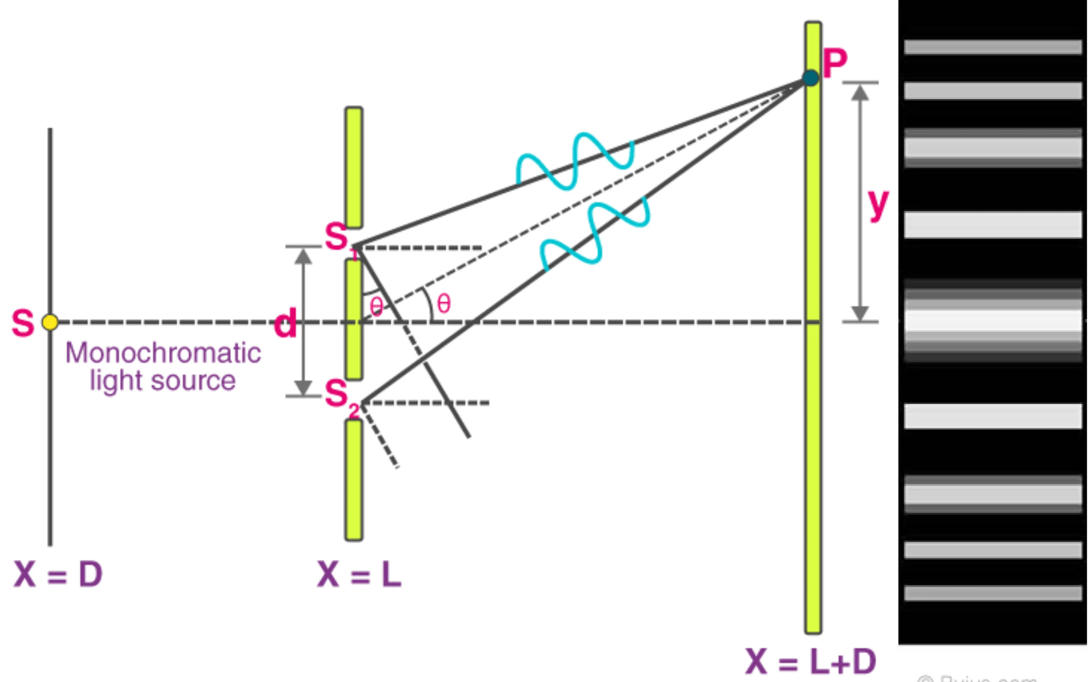
4.1 Young's Double Slit Experiment

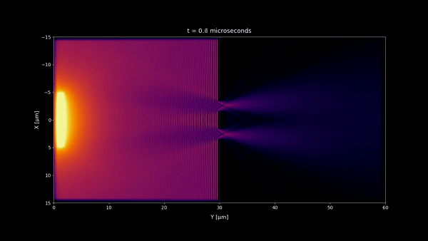
Let us first consider the famous Young's double-slit experiment, where light from a source is diffracted by two narrow, parallel slits of the same width:

Attachments/Notes/2025 Quantum Electronics/4 Coherence and Interference/02_Fundamental_phenomena.webp|700

Coherent light
First, the simulation is performed with coherent light, idealised as a Gaussian beam, which is a common approximation for the output of a single-mode laser. For now, consider this light as perfectly coherent because its bandwidth is effectively zero; that is to say, it is perfectly monochromatic light:

Attachments/Notes/2025 Quantum Electronics/4 Coherence and Interference/coherent 1.gif|700

As we can see, the beam passes through the slits and produces an interference pattern on a screen, which is stationary over typical observation timescales.

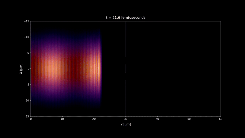
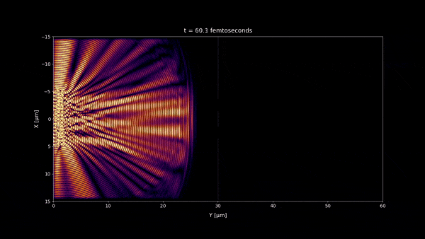
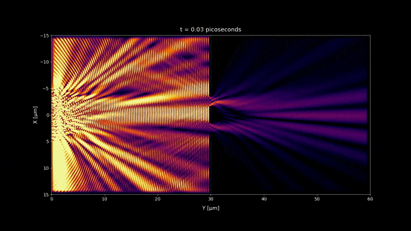
Incoherent Light
On the other hand, consider the same experiment with spatially incoherent light, such as light with a finite spectral bandwidth and finite spatial extent, observed over three different timescales:

Attachments/Notes/2025 Quantum Electronics/4 Coherence and Interference/simulation-incoherent-femtoseconds.gif|700
(Femtosecond timescale)

Attachments/Notes/2025 Quantum Electronics/4 Coherence and Interference/simulation-incoherent-picoseconds.gif|700
(Picosecond timescale)

Attachments/Notes/2025 Quantum Electronics/4 Coherence and Interference/simulation-incoherent-microseconds.gif|700
(Microsecond timescale)

We observe that the interference pattern fluctuates significantly, particularly evident on the picosecond timescale in this simulation. As we will see later, this timescale is related to the light's coherence time $τ_{c}$ , which for this example with a given centre wavelength $λ_{0}$ and spectral bandwidth $Δ λ$ , can be estimated as:

τ_{c} \sim \frac{λ_{0}^{2}}{c Δ λ} .

For typical parameters used in such simulations (for instance, $λ_{0} = 800 nm$ , $Δ λ = 0.37 nm$ ), this yields $τ_{c} \approx 1.4 ps$ .

4.2 Coherence Function

Let us define coherence—'the ability to interfere'—more precisely. To this end, we introduce the mutual (first-order) coherence function, which correlates an electric field $E$ with itself at different positions and times:

Γ (r_{1}, t_{1}; r_{2}, t_{2}) = ⟨ E^{*} (r_{1}, t_{1}) \cdot E (r_{2}, t_{2}) ⟩ .

The angle brackets $⟨ \cdot ⟩$ denote an ensemble average over many realisations of the field, reflecting the statistical properties of the light source, particularly for partially coherent or random light. This averaging accounts for fluctuations in the optical fields. For ergodic fields, this ensemble average can be replaced by a time average. In this context, coherence describes how reproducible an interference pattern is.

We generally differentiate between two types of coherence:

Transverse or spatial coherence: Characterised by $Γ (r_{1}, t; r_{2}, t)$ , considering correlation at the same time $t$ but different positions.
Longitudinal or temporal coherence: Characterised by $Γ (r, t_{1}; r, t_{2})$ , considering correlation at the same position $r$ but different times.

We will often work with statistically stationary fields, meaning fields whose statistical properties (like the mean and autocorrelation) do not change over time. For first-order stationarity, $⟨ E (r, t) ⟩$ is constant (often zero for optical fields). For second-order stationarity relevant here, the mutual coherence function depends only on the time difference $τ = t_{2} - t_{1}$ , not on absolute times $t_{1}, t_{2}$ :

Γ (r_{1}, r_{2}, τ) = ⟨ E^{*} (r_{1}, t) \cdot E (r_{2}, t + τ) ⟩ .

From this, we define the temporal (auto)coherence function (or self-coherence function) at a single point $r$ as:

G (r, τ) = Γ (r, r, τ) = ⟨ E^{*} (r, t) \cdot E (r, t + τ) ⟩ .

For simplicity, if position is fixed, we write $G (τ)$ . Perhaps more important is the normalised version, the complex degree of (temporal) coherence:

g (τ) = \frac{G (τ)}{G (0)},

where $G (0) = ⟨ | E (r, t) |^{2} ⟩$ is proportional to the average intensity. The magnitude $| g (τ) |$ ranges from $0$ (incoherent) to $1$ (perfectly coherent).

We can broadly distinguish two limiting cases:

High coherence (for instance, an ideal laser): The phase relationship between the field at time $t$ and $t + τ$ is perfectly deterministic for all $τ$ . Thus, $| g (r, τ) | = 1$ for all $τ$ .
Low coherence (for instance, an idealised thermal lightbulb): The phase relationship between $t$ and $t + τ$ becomes rapidly decorrelated for $τ \neq 0$ . Thus, $| g (r, τ) | \to 0$ for $τ ≫ τ_{c}$ (coherence time).

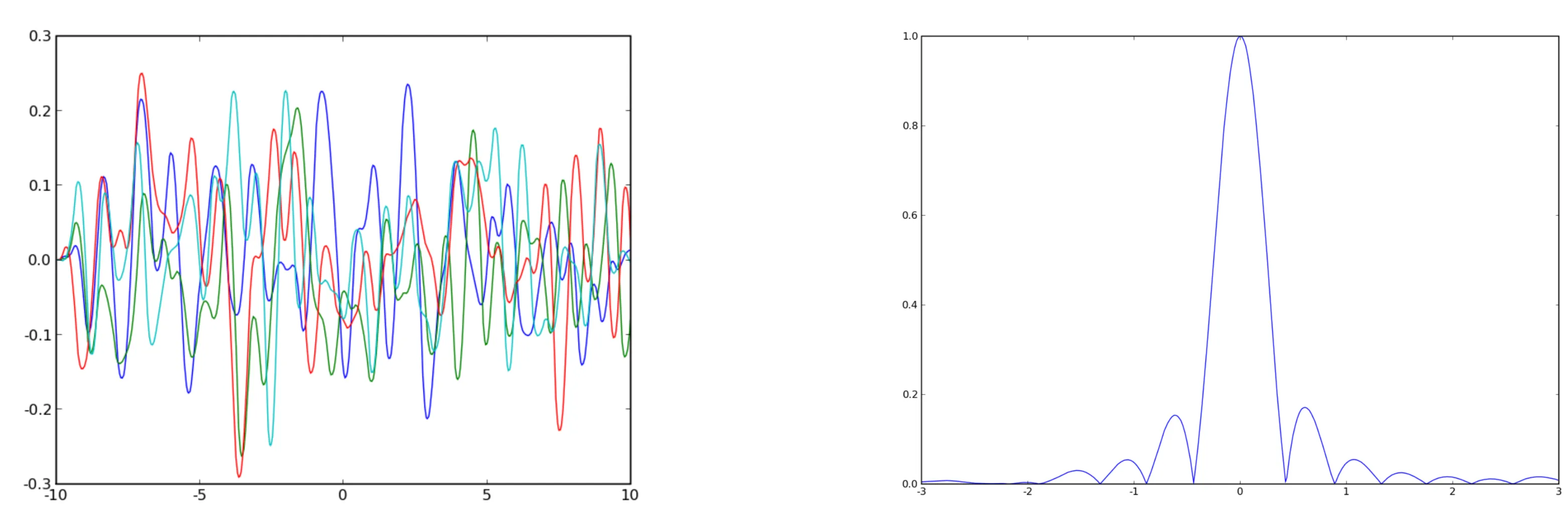
Let us consider a concrete example: a superposition of monochromatic plane waves, all of the same frequency $ω$ and amplitude $E_{0}$ , but each with a random, statistically independent phase $φ_{j}$ . If we consider a single such wave train $E_{j} (t) = E_{0} e^{i (ω t + φ_{j})}$ , its autocorrelation (if $φ_{j}$ is fixed for this train) would be:

\begin{aligned} G_{j} (τ) & = {⟨ {(E_{0} e^{i (ω t + φ_{j})})}^{*} \cdot (E_{0} e^{i (ω (t + τ) + φ_{j})}) ⟩}_{time or fixed phase} \\ = E_{0}^{*} \cdot E_{0} e^{i ω τ} = | E_{0} |^{2} e^{i ω τ} . \end{aligned}

For this ideal monochromatic wave, the complex degree of coherence is:

g (τ) = \frac{G (τ)}{G (0)} = \frac{| E_{0} |^{2} e^{i ω τ}}{| E_{0} |^{2}} = e^{i ω τ} ⟹ | g (τ) | = 1 for all τ .

Since $| g (τ) |$ cannot exceed $1$ , this represents maximum temporal coherence. Such a signal allows prediction of its phase at any time from knowledge of its phase at any other time.

In comparison, consider light composed of many such wave trains where the phases $φ_{j}$ are random and uncorrelated from one train to the next (a more realistic model for some types of partially coherent light). The ensemble average $⟨ e^{i (φ_{k} - φ_{j})} ⟩$ would be non-zero only if $j = k$ . For a truly random (delta-correlated in time or "white noise" like) field, the coherence function approaches a delta function:

Attachments/Notes/2025 Quantum Electronics/4 Coherence and Interference/QE_script 11.webp|700

We find that, for such a highly random field,

| g (τ) | \to 0, for | τ | ≫ τ_{c} where τ_{c} is very small .

Therefore, $g (τ)$ is sharply peaked around $τ = 0$ , being $1$ at zero time delay and decaying rapidly for non-zero delays.

4.3 Coherence Time and Coherence Length

The concept of coherence allows us to define a characteristic coherence time $τ_{c},$ which quantifies the temporal interval over which the field remains significantly correlated with itself. One common definition is:

τ_{c} = \int_{- \infty}^{\infty} | g (τ) |^{2} d τ .

The coherence time is inversely proportional to the spectral bandwidth $Δ f$ (or $Δ ν$ ) of the light source, a relationship that stems from Fourier theory (specifically, the Wiener-Khinchin theorem discussed next):

τ_{c} \sim \frac{1}{Δ f} .

Therefore, the example of ideal monochromatic plane waves (zero bandwidth) yields an infinite coherence time, while truly random (white noise) fields (infinite bandwidth) would have a zero coherence time.
Similarly, we define the coherence length $l_{c}$ as the distance over which light maintains a significant degree of coherence:

l_{c} = c τ_{c},

where $c$ is the speed of light in vacuum. For unfiltered sunlight, $τ_{c}$ is roughly $1 - 2 fs$ , corresponding to $l_{c} \approx 300 - 600 nm$ . In contrast, a highly stabilised single-mode laser can have a coherence time of milliseconds or even seconds, implying a coherence length of hundreds to thousands of kilometres.

4.4 Wiener-Khinchin Theorem

First, we define the Power Spectral Density (PSD), denoted $S (ω)$ , of a stationary random process $E (t)$ . For a truncated version of the signal $E_{T} (t)$ (equal to $E (t)$ for $- T / 2 \leq t \leq T / 2$ and zero otherwise), let $V_{T} (ω)$ be its Fourier transform:

V_{T} (ω) = \int_{- T / 2}^{T / 2} E (t) e^{- i ω t} d t .

The PSD is then defined as:

S (ω) = lim_{T \to \infty} \frac{1}{2 π T} ⟨ {| V_{T} (ω) |}^{2} ⟩ .

The PSD describes the distribution of the average power of the signal over frequency, usually specified in units such as milliwatts per terahertz, although "power" here refers to the power of a signal in a general sense ( $| E |^{2}$ ), not necessarily optical power in Watts.
The Wiener-Khinchin theorem then states that the Power Spectral Density $S (ω)$ of a wide-sense stationary random process is the Fourier transform of its autocorrelation function $G (τ)$ :

S (ω) = \frac{1}{2 π} \int_{- \infty}^{\infty} G (τ) e^{- i ω τ} d τ .

Conversely, $G (τ)$ is the inverse Fourier transform of $2 π S (ω)$ . This theorem provides a fundamental link between the time-domain coherence properties of a signal ( $G (τ)$ ) and its frequency-domain spectral properties ( $S (ω)$ ). From this, it is clear that there must also be a relationship between the coherence time $τ_{c}$ (related to the width of $G (τ)$ or $| g (τ) |$ ) and the spectral width $Δ ω$ (or $Δ f$ , the FWHM of $S (ω)$ ).
Next, some examples of coherence properties for various light sources are shown:

Source	$Δ f_{c} (Hz)$	$τ_{c} \approx 1 / Δ f_{c}$	$l_{c} = c τ_{c}$
Unfiltered sunlight ( $λ_{0} \approx 0.4 - 0.8 μ m$ , $Δ λ \approx 0.4 μ m$ )	$\sim 3.75 \times 10^{14}$	$\sim 2.7 fs$	$\sim 800 nm$
Light emitting diode ( $λ_{0} = 1 μ m, Δ λ_{0} = 50 nm$ )	$\sim 1.5 \times 10^{13}$	$\sim 67 fs$	$\sim 20 μ m$
Low-pressure sodium lamp	$\sim 5 \times 10^{11}$	$\sim 2 ps$	$\sim 600 μ m$
Multi-mode He-Ne laser ( $λ_{0} = 633 nm$ )	$\sim 1.5 \times 10^{9}$	$\sim 0.67 ns$	$\sim 20 cm$
Single-mode He-Ne laser ( $λ_{0} = 633 nm$ )	$\sim 1 \times 10^{6}$	$\sim 1 μ s$	$\sim 300 m$

4.5 Interference

Naturally, the next question is how we measure temporal coherence properties. This is commonly done with interferometric setups. The most common one is the Michelson interferometer. The basic idea of all such two-beam interferometers is to split a light beam into two replicas, guide them along different optical paths (introducing a relative time delay), recombine them, and measure the intensity of the resulting superposed wave, for instance using a photodiode or bolometer. As stated, coherence is often described as the ability of light to interfere; therefore, it is natural to measure light's ability to interfere with a time-delayed version of itself.

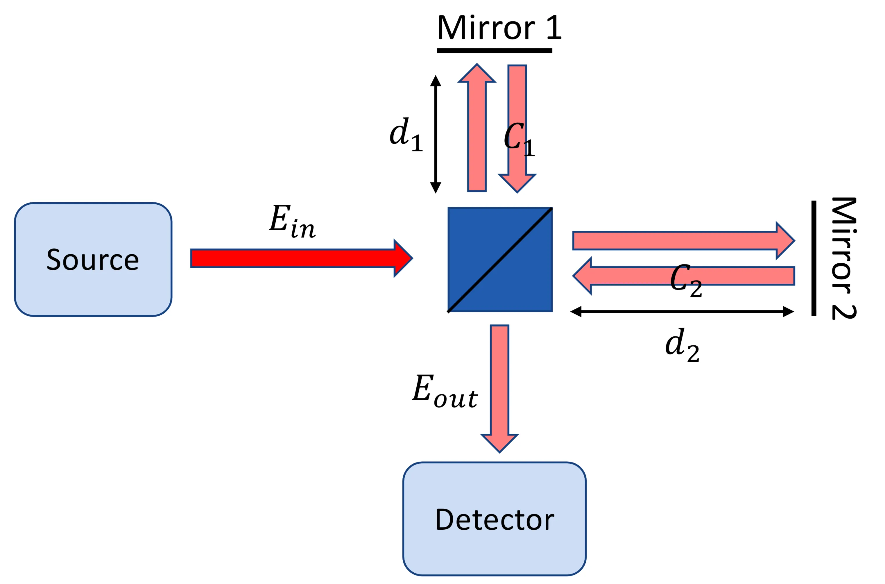
4.5.1 (Michelson) Interferometer

Consider the following Michelson interferometer setup, where incoming light is split into two replicas by a beam splitter. We assume no change in polarisation state occurs.

Attachments/Notes/2025 Quantum Electronics/4 Coherence and Interference/02_Fundamental_phenomena 2.webp|700

The output electric field at the detector can be written as a superposition of the fields from the two arms:

E_{out} (t) = C_{1} E_{in} (t - τ_{1}) + C_{2} E_{in} (t - τ_{2}),

where $C_{1}, C_{2}$ are complex constants accounting for reflection/transmission coefficients and propagation losses in each arm, and $τ_{1}, τ_{2}$ are the respective time delays. The measured average intensity is $I_{out} = \frac{1}{2 Z_{0}} ⟨ | E_{out} (t) |^{2} ⟩$ (assuming impedance $Z_{0}$ and scalar fields for simplicity):

\begin{aligned} I_{out} & \sim ⟨ {| C_{1} E_{in} (t - τ_{1}) + C_{2} E_{in} (t - τ_{2}) |}^{2} ⟩ \\ = ⟨ (C_{1} E_{in} (t - τ_{1}) + C_{2} E_{in} (t - τ_{2})) \cdot (C_{1}^{*} E_{in}^{*} (t - τ_{1}) + C_{2}^{*} E_{in}^{*} (t - τ_{2})) ⟩ \\ = | C_{1} |^{2} ⟨ | E_{in} (t - τ_{1}) |^{2} ⟩ + | C_{2} |^{2} ⟨ | E_{in} (t - τ_{2}) |^{2} ⟩ \\ + C_{1} C_{2}^{*} ⟨ E_{in} (t - τ_{1}) E_{in}^{*} (t - τ_{2}) ⟩ + C_{1}^{*} C_{2} ⟨ E_{in}^{*} (t - τ_{1}) E_{in} (t - τ_{2}) ⟩ . \end{aligned}

For stationary fields, $⟨ | E_{in} (t - τ_{1}) |^{2} ⟩ = ⟨ | E_{in} (t - τ_{2}) |^{2} ⟩ = G (0) \sim I_{in}$ .
Also, $⟨ E_{in}^{*} (t - τ_{1}) E_{in} (t - τ_{2}) ⟩ = G (τ_{2} - τ_{1})$ . So the cross terms become $C_{1} C_{2}^{*} G^{*} (τ_{1} - τ_{2}) + C_{1}^{*} C_{2} G (τ_{1} - τ_{2}) = 2 Re [C_{1}^{*} C_{2} G (τ_{1} - τ_{2})]$ .
Thus, letting $τ = τ_{1} - τ_{2}$ :

I_{out} (τ) = I_{1} + I_{2} + 2 \sqrt{I_{1} I_{2}} Re [g (τ) e^{i α_{12}}],

where $I_{1} \sim | C_{1} |^{2} I_{in}$ , $I_{2} \sim | C_{2} |^{2} I_{in}$ , and $e^{i α_{12}}$ accounts for relative phases from $C_{1}, C_{2}$ . If we normalise, and define $g (τ) = G (τ) / G (0)$ :

I_{out} (τ) \sim | C_{1} |^{2} G (0) + | C_{2} |^{2} G (0) + 2 Re [C_{1}^{*} C_{2} G (0) g (τ)] .

This shows that we can obtain information about $Re [g (τ)]$ by measuring the output intensity of an interferometer as a function of the relative delay $τ = τ_{1} - τ_{2}$ . The interference term is non-zero as long as $| τ_{1} - τ_{2} |$ is within the coherence time $τ_{c}$ . For a 50:50 beam splitter where $| C_{1} | = | C_{2} | = C$ (assuming equal path losses other than delay), we get:

I_{out} (τ) = 2 | C |^{2} I_{in} (1 + Re [g (τ) e^{i ϕ_{12}}]),

where $ϕ_{12}$ is the phase of $C_{1}^{*} C_{2}$ .
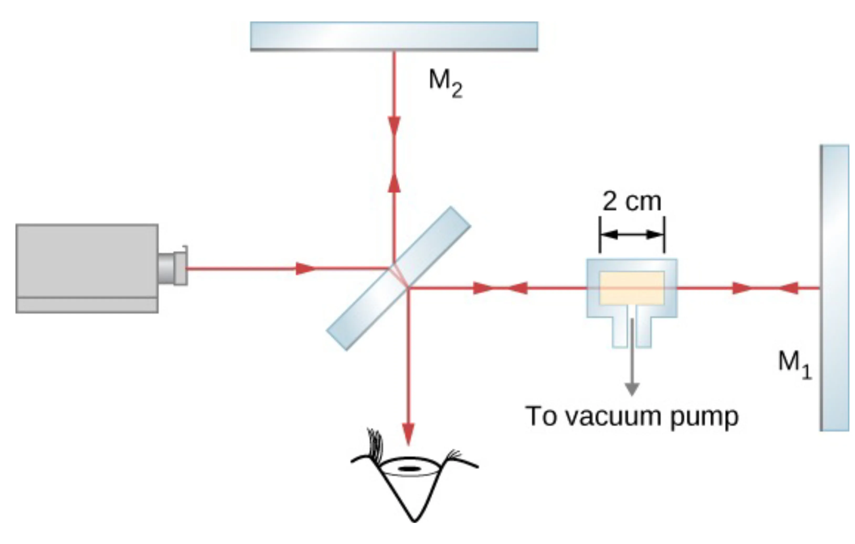
This setup allows precise measurement of optical path length differences via fringe counting, as used in gravitational wave detectors like LIGO, capable of detecting angstrom-scale changes in kilometre-long arm lengths. A slight modification allows measurement of the refractive index of a gas:

Attachments/Notes/2025 Quantum Electronics/4 Coherence and Interference/02_Fundamental_phenomena 3.webp|700

Assuming the gas cuvette has length $Δ x$ , the relative time delay introduced by the gas is related to its refractive index $n_{gas}$ compared to the reference path (perhaps air, $n_{air}$ ). If arm 2 contains the cuvette and arm 1 is reference:

τ = τ_{1} - τ_{2} = \frac{2 d_{1} n_{ref}}{c} - \frac{2 ((d_{2} - Δ x) n_{ref} + Δ x n_{gas})}{c} .

By varying the gas pressure (and thus $n_{gas}$ ) and observing the shift in interference fringes, $n_{gas}$ can be determined.
This interferometric setup, when used to measure $G (τ)$ or $g (τ)$ and then applying the Wiener-Khinchin theorem, allows one to obtain the power spectral density $S (ω)$ without using a traditional spectrometer. This technique is known as Fourier Transform Spectroscopy (FTS), particularly Fourier Transform Infrared Spectroscopy (FTIR) when applied in the infrared.
Regarding the complex nature of $g (τ)$ : $S (ω)$ must be real and non-negative. Since $G (τ)$ is an autocorrelation function, $G (- τ) = G^{*} (τ)$ , which ensures $S (ω)$ is real. Both magnitude and phase of $g (τ)$ are generally needed to fully characterise the coherence. The real part $Re [g (τ)]$ determines the observed fringe pattern in a simple intensity measurement.

4.6 Fabry-Pérot Interferometer - Etalon

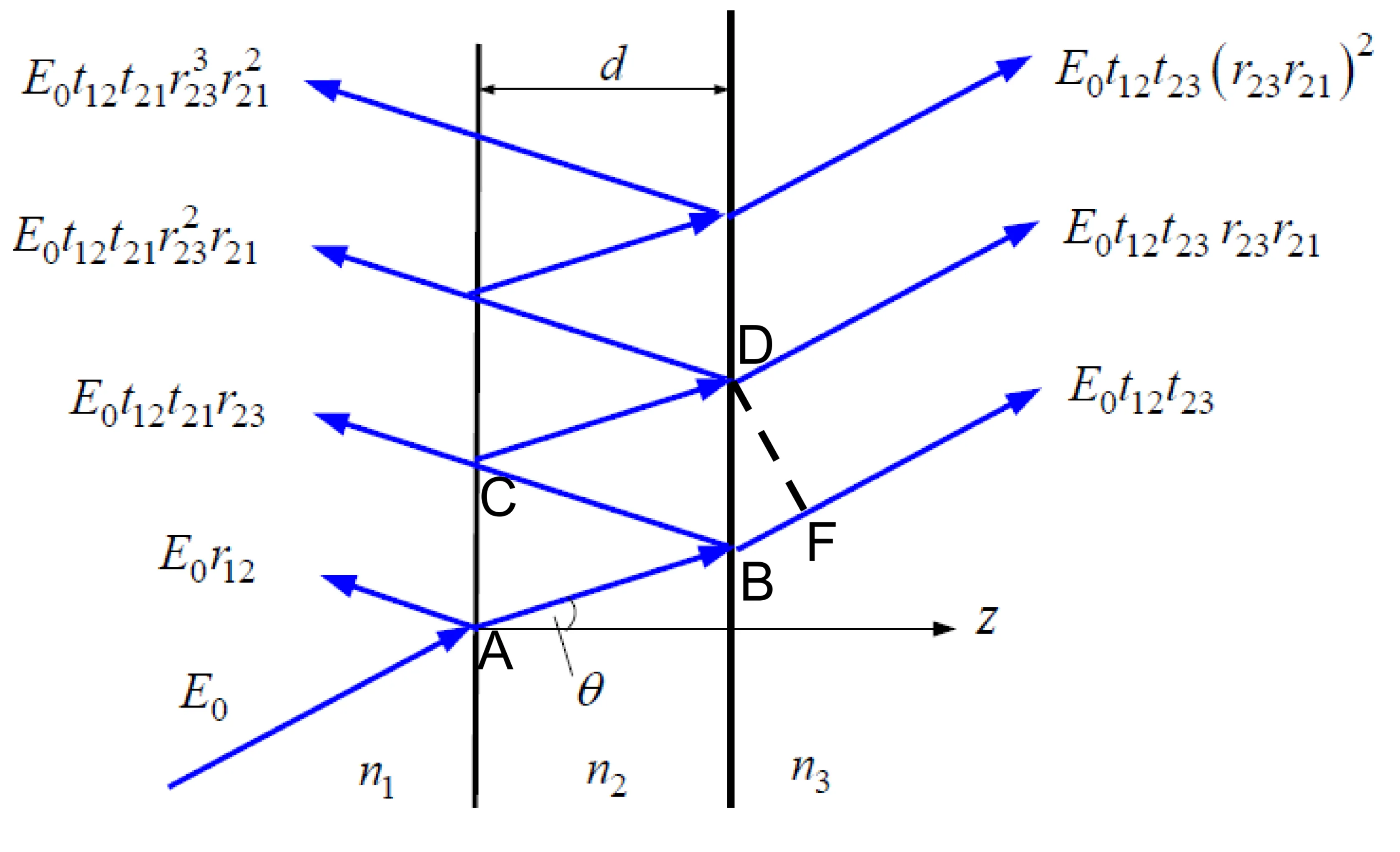
Consider a thin film of material of refractive index $n_{2}$ and thickness $d$ , surrounded by media with refractive indices $n_{1}$ (incident side) and $n_{3}$ (transmitting side). This forms a Fabry-Pérot etalon.

Attachments/Notes/2025 Quantum Electronics/4 Coherence and Interference/02_Fundamental_phenomena 4.webp|700

Assume a plane light wave $E_{0}$ is incident from medium 1. It is multiply reflected and transmitted at the interfaces. Summing all transmitted partial waves (taking into account phase shifts from propagation and phase changes upon reflection), we find the total transmitted field $E_{t}$ :

\begin{aligned} E_{t} & = E_{0} t_{12} t_{23} e^{i ϕ} + E_{0} t_{12} r_{23} r_{21} t_{23} e^{i 3 ϕ} + E_{0} t_{12} (r_{23} r_{21})^{2} t_{23} e^{i 5 ϕ} + \dots \\ = E_{0} t_{12} t_{23} e^{i ϕ} \sum_{m = 0}^{\infty} (r_{21} r_{23} e^{i 2 ϕ})^{m} = E_{0} \frac{t_{12} t_{23} e^{i ϕ}}{1 - r_{21} r_{23} e^{i 2 ϕ}} . \end{aligned}

Here $t_{i j}$ and $r_{i j}$ are the amplitude transmission and reflection coefficients for a wave incident from medium $i$ towards medium $j$ . The single-pass phase accumulation across the layer of thickness $d$ at an internal angle $θ_{2}$ is $ϕ = k_{2 z} d = (n_{2} ω / c) \cos θ_{2} d$ . The round-trip phase is $2 ϕ$ . Similarly, for the reflected part $E_{r}$ :

r_{FP} = \frac{E_{r}}{E_{0}} = r_{12} + \frac{t_{12} r_{23} t_{21} e^{i 2 ϕ}}{1 - r_{21} r_{23} e^{i 2 ϕ}} .

The transmission coefficient for the Fabry-Pérot etalon is $t_{FP} = E_{t} / E_{0}$ . Assuming the $e^{i ϕ}$ factor for single pass is part of $t_{23}$ or overall definition, then:

t_{FP} = \frac{t_{12} t_{23}}{1 - r_{21} r_{23} e^{i 2 ϕ}} .

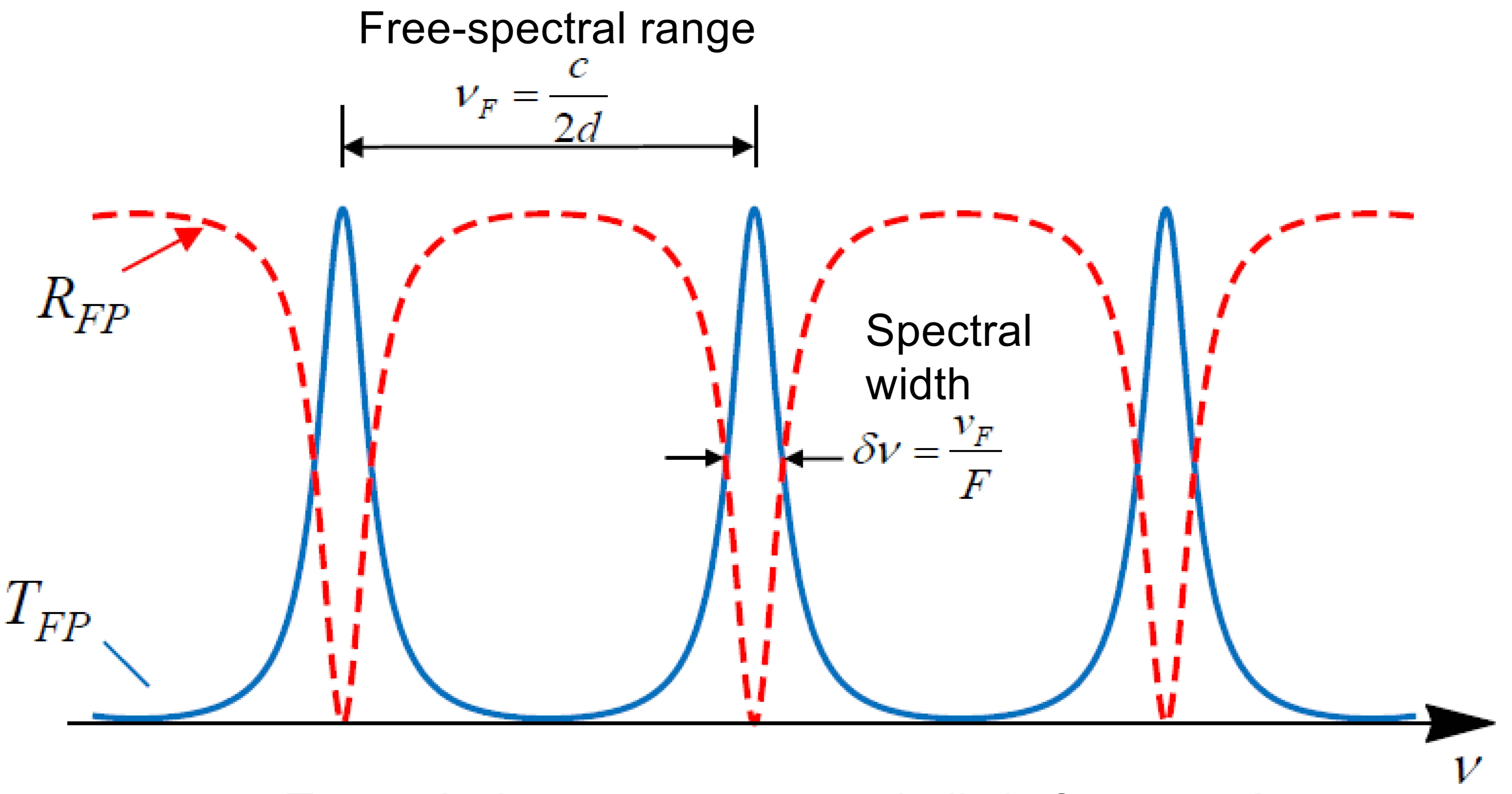
The power transmittance $T_{FP} = | t_{FP} |^{2}$ can be written as:

T_{FP} = \frac{| t_{12} |^{2} | t_{23} |^{2}}{| 1 - r_{21} r_{23} e^{i 2 ϕ} |^{2}} = \frac{T_{12} T_{23}}{(1 - \sqrt{R_{12} R_{23}})^{2} + 4 \sqrt{R_{12} R_{23}} \sin^{2} (ϕ + δ_{21} / 2 + δ_{23} / 2)},

where $R_{i j} = | r_{i j} |^{2}$ , $T_{i j} = | t_{i j} |^{2},$ and $δ_{i j}$ are phases of $r_{i j}$ . Another common way to write this is

T_{FP} = {| t_{FP} |}^{2} = \frac{{| t_{12} t_{23} |}^{2}}{{| 1 - r_{23} r_{21} e^{i 2 ϕ} |}^{2}} = \frac{T_{FPmax}}{1 + {(\frac{2 F}{π})}^{2} \sin^{2} ϕ},

where $T_{FPmax} = \frac{| t_{12} t_{23} |^{2}}{(1 - | r_{23} r_{21} |)^{2}}$ and $F = \frac{π \sqrt{| r_{12} r_{23} |}}{1 - | r_{23} r_{21} |}$ . The Finesse $F$ relates the free spectral range (FSR) to the resonance linewidth.

Attachments/Notes/2025 Quantum Electronics/4 Coherence and Interference/02_Fundamental_phenomena 5.webp|700

The transmission as a function of optical frequency $f$ (where $2 ϕ = 2 π f / f_{FSR}$ , with $f_{FSR} = c / (2 n_{2} d \cos θ_{2})$ being the free spectral range):

T_{FP} (f) = \frac{T_{FPmax}}{1 + {(\frac{2 F}{π})}^{2} \sin^{2} (π \frac{f}{f_{FSR}})} .

The FSR is determined by the optical path length of the cavity, whereas the finesse $F$ is primarily determined by the reflectivity of the interfaces.

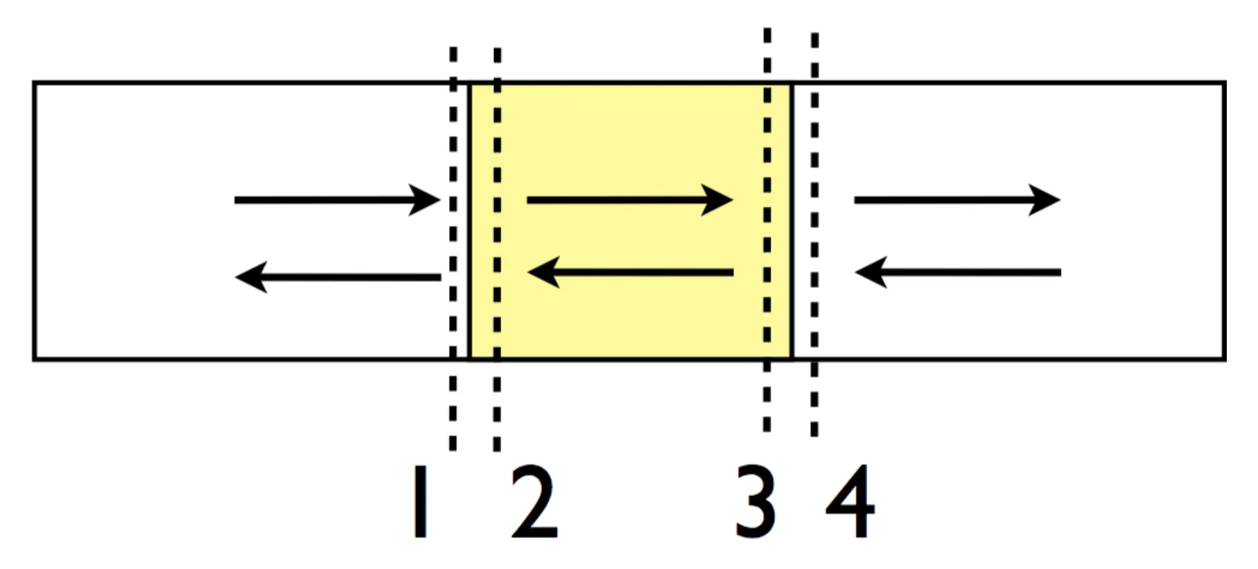
4.7 Matrix Methods for Multiple Surfaces

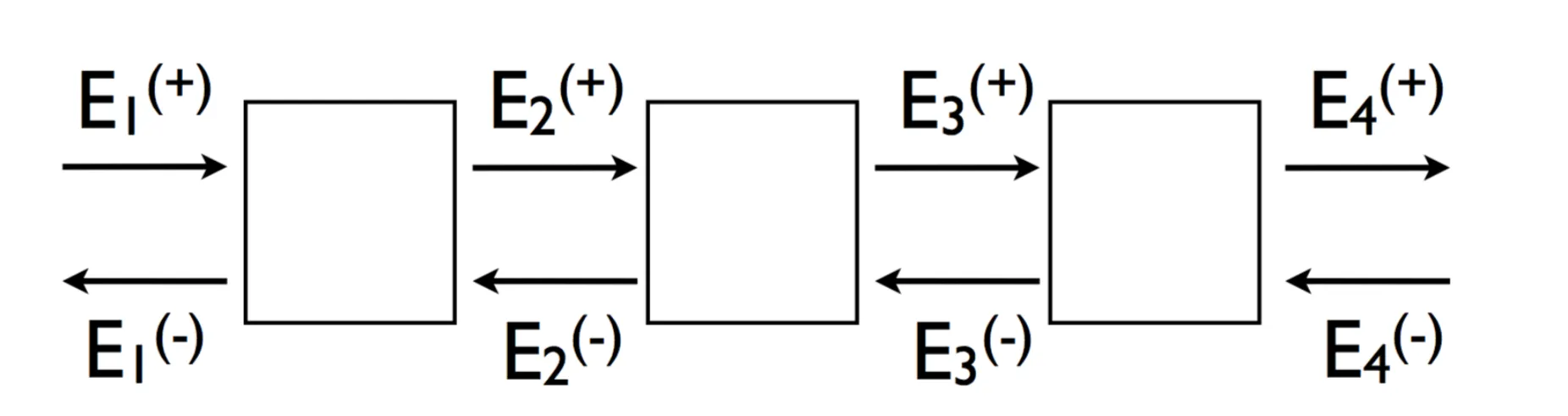
Consider an optical system composed of multiple elements or interfaces.

Attachments/Notes/2025 Quantum Electronics/4 Coherence and Interference/QE_script 12.webp|700

Each box represents an optical element modifying the electric field amplitude and phase. We consider light propagating along a single axis and only one polarisation (s- or p-polarised light). The superscripts $(+)$ and $(-)$ indicate whether the wave propagates to the right or the left, respectively, at a reference plane.

Attachments/Notes/2025 Quantum Electronics/4 Coherence and Interference/QE_script 13.webp|700

At interface 1 (between medium 0 and 1, fields in medium 1 are $E_{1}^{(+)}, E_{1}^{(-)}$ ), we define a matrix relating fields on one side of an element/interface to the other. The transfer matrix (or ABCD matrix for a system) relates fields at the output plane (say, plane 2) to fields at the input plane (plane 1):

(\begin{matrix} E_{1}^{(+)} \\ E_{1}^{(-)} \end{matrix}) = M_{12} (\begin{matrix} E_{2}^{(+)} \\ E_{2}^{(-)} \end{matrix}) = (\begin{matrix} A_{12} & B_{12} \\ C_{12} & D_{12} \end{matrix}) (\begin{matrix} E_{2}^{(+)} \\ E_{2}^{(-)} \end{matrix}) .

For a cascade of elements from plane 1 to plane $N + 1$ :

(\begin{matrix} E_{1}^{(+)} \\ E_{1}^{(-)} \end{matrix}) = M_{12} M_{23} \dots M_{N, N + 1} (\begin{matrix} E_{N + 1}^{(+)} \\ E_{N + 1}^{(-)} \end{matrix}) = M_{total} (\begin{matrix} E_{N + 1}^{(+)} \\ E_{N + 1}^{(-)} \end{matrix}) .

Then for the system from 1 to 4:

(\begin{matrix} E_{4}^{(+)} \\ E_{4}^{(-)} \end{matrix}) = M_{34} M_{23} M_{12} (\begin{matrix} E_{1}^{(+)} \\ E_{1}^{(-)} \end{matrix}) = (\begin{matrix} A_{14} & B_{14} \\ C_{14} & D_{14} \end{matrix}) (\begin{matrix} E_{1}^{(+)} \\ E_{1}^{(-)} \end{matrix}) .

These are wave-propagation (transfer) matrices.

Propagation in uniform medium of length $d$ :
The matrix relating fields at $z = 0$ ( $E_{1}$ ) to fields at $z = d$ ( $E_{2}$ ) is:

(\begin{matrix} E_{2}^{(+)} \\ E_{2}^{(-)} \end{matrix}) = (\begin{matrix} e^{- i k d} & 0 \\ 0 & e^{i k d} \end{matrix}) (\begin{matrix} E_{1}^{(+)} \\ E_{1}^{(-)} \end{matrix}) .

This means $E_{2}^{(+)} = E_{1}^{(+)} e^{- i k d}$ (forward wave accumulates phase) and $E_{2}^{(-)} = E_{1}^{(-)} e^{i k d} .$

Scattering matrix (S-matrix) relates outgoing waves to incoming waves:

(\begin{matrix} E_{1}^{(-)} \\ E_{2}^{(+)} \end{matrix}) = (\begin{matrix} r_{12} & t_{21} \\ t_{12} & r_{21} \end{matrix}) (\begin{matrix} E_{1}^{(+)} \\ E_{2}^{(-)} \end{matrix}) .

This means $E_{1}^{(-)} = r_{12} E_{1}^{(+)} + t_{21} E_{2}^{(-)}$ (reflection from and transmission into port 1) and $E_{2}^{(+)} = t_{12} E_{1}^{(+)} + r_{21} E_{2}^{(-)}$ (transmission into and reflection from port 2).

Relation between Transfer (ABCD) and Scattering (S) matrices:
If $S = (\begin{matrix} s_{11} & s_{12} \\ s_{21} & s_{22} \end{matrix})$ , then the transfer matrix $M$ such that $(\begin{matrix} E_{1}^{(+)} \\ E_{1}^{(-)} \end{matrix}) = M (\begin{matrix} E_{2}^{(+)} \\ E_{2}^{(-)} \end{matrix})$ is often given as $M = (\begin{matrix} s_{21}^{- 1} & - s_{21}^{- 1} s_{22} \\ s_{11} s_{21}^{- 1} & s_{12} - s_{11} s_{21}^{- 1} s_{22} \end{matrix})$ .

4.7.1 Properties of the Scattering Matrix

Lossless system: $S^{†} S = I$ (unitary).
Reciprocal system: $S = S^{T}$ ( $S_{12} = S_{21}$ ).