Jump back to chapter selection.

Table of Contents

2.1 Origin of Dispersion
2.2 Kramers-Kronig Relations
2.3 Equations in Frequency Domain
2.4 Helmholtz Equation
2.5 Refractive Index in Dispersive Media
2.6 Light Pulses
2.7 Time-Bandwidth Product of Wavepackets
2.8 Phase, Group and Front Velocity

2 Propagation in Dispersive Media

Thinking back to approximation 4 in Chapter 1, we assumed that the polarisation and magnetisation depend linearly on the instantaneous values of the electric and magnetic fields. However, as we noted, this is only true for slow changes in the fields with time and cannot be entirely true for rapidly oscillating fields. In other words, we assumed the system (material) to have no memory. This assumption implies an absence of dispersion, as we will see soon. While it seems obvious that the polarisation and magnetisation cannot depend on future field values (causality), real materials do possess some limited memory of past fields:

Intuitively, consider that the electric field creates a polarisation by inducing an oscillation of the bound electrons in the atoms of the medium, collectively producing the polarisation density. A time delay between cause ($\mathbf{E}$) and effect ($\mathbf{P}$) arises from the finite response time of the atoms; they cannot react infinitely fast to sudden changes in the applied fields.

With our prior assumption of an instantaneous response, we were able to drop the integral in the general response function. This is no longer the case for dispersive media. For a linear, causal system, the response is a convolution in the time domain:

Here, ${\chi }_e(t)$ and ${\chi }_m(t)$ are the time-dependent electric and magnetic susceptibility response functions, respectively. Causality requires ${\chi }_e(\tau )=0$ and ${\chi }_m(\tau )=0$ for $\tau <0$. The presence of these convolution integrals signifies that the material has memory.
A significant advantage of Fourier transformation is that convolution in the time domain becomes simple multiplication in the frequency domain. The above equations are equivalent to:

The frequency-dependent susceptibilities ${\chi }_e(\omega )$ and ${\chi }_m(\omega )$ are generally complex quantities. Their form is analogous to the transfer function in linear systems theory: the response ($\mathbf{P}(\omega )$ or $\mathbf{M}(\omega )$) is the product of the input signal spectrum ($\mathbf{E}(\omega )$ or $\mathbf{H}(\omega )$) and the system's transfer function (the susceptibility). We can now properly define dispersion: Dispersion means that the material response function (susceptibility, and thus permittivity or permeability) depends on frequency.

To understand the meaning of a complex susceptibility, consider applying a real electric field $\mathbf{E}(t)={\mathbf{E}}_0\cos \left({\omega }_{0}t\right)$ to a medium. The Fourier transform of this field is:

With the frequency-domain relation $\mathbf{P}(\omega )={\epsilon }_0{\chi }_e(\omega )\mathbf{E}(\omega )$, we obtain the polarisation spectrum:

Transforming back to the time domain gives the polarisation as a function of time:

Since the impulse response ${\chi }_e(t)$ must be real for a physical system responding to a real field $\mathbf{E}(t)$ with a real polarisation $\mathbf{P}(t)$, its Fourier transform ${\chi }_e(\omega )$ must satisfy the conjugate symmetry property ${\chi }_e(-{\omega }_0)={\chi }_e^{\ast }({\omega }_0)$. Thus,

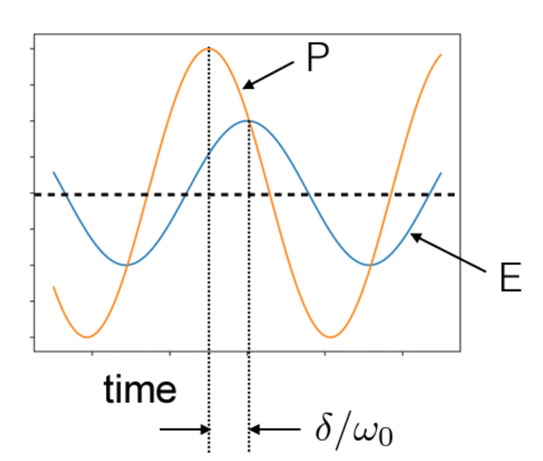
Therefore, $|{\chi }_e({\omega }_0)|$ relates the amplitude of the polarisation density response $P_0$ to the applied electric field amplitude $E_0$ (as $P_0={\epsilon }_0|{\chi }_e({\omega }_0)|E_0$), while the phase of the complex ${\chi }_e({\omega }_0)$ introduces a phase shift between the polarisation $\mathbf{P}(t)$ and the driving field $\mathbf{E}(t)$. This is shown in the next figure:

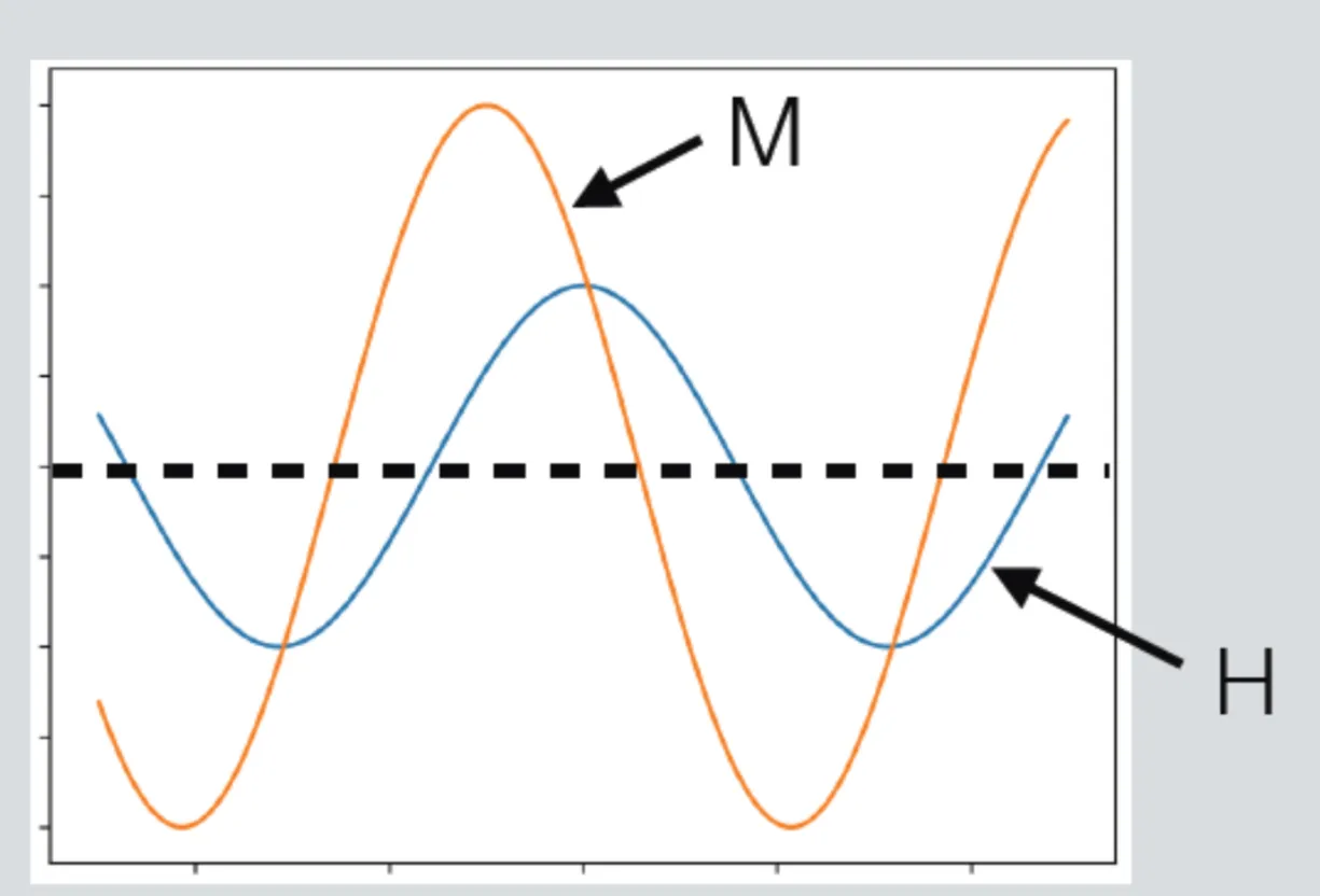
Similarly, for the magnetisation response to an applied magnetic field $\mathbf{H}(t)={\mathbf{H}}_0\cos ({\omega }_{0}t)$:

This is shown in the next figure:

We will later see that the imaginary part of the susceptibility, $\mathfrak{Im}[{\chi }_e(\omega )]$, is related to absorption or gain of electromagnetic energy in the medium.

2.1 Origin of Dispersion

2.1.1 Drude-Lorentz model

Let us start with a simple classical model, where we treat an electron in an atom (or a bound charge carrier) as being connected by a spring to a much heavier, effectively immobile ion core. We assume the electron mass is $m_e$. The equation of motion for the displacement $x$ of the electron from its equilibrium position, driven by an external electric field and subject to damping, is that of a simple damped harmonic oscillator:

Here, ${\omega }_0$ is the natural resonance frequency of the oscillator, and $\gamma$ is a damping coefficient representing energy loss mechanisms. The driving force is $F(t)=-eE(t)$, where $-e$ is the charge of the electron and $E(t)$ is the local electric field experienced by the electron.
The induced dipole moment for one such oscillator is $p(t)=-ex(t)$. If there are $N$ such oscillators per unit volume, the macroscopic polarisation density is $P(t)=Np(t)=-Nex(t)$. Substituting $x(t)=-P(t)/(Ne)$, the equation of motion for $P(t)$ becomes:

Next, we Fourier transform this equation (assuming $E(t)\leftrightarrow E(\omega )$ and $P(t)\leftrightarrow P(\omega )$ with $\partial /\partial t\leftrightarrow i\omega$ for fields like $e^{i\omega t}$):

This allows us to solve for $P(\omega )$ in terms of $E(\omega )$ and thus find the electric susceptibility ${\chi }_e(\omega )=P(\omega )/({\epsilon }_{0}E(\omega ))$:

where the static susceptibility ${\chi }_0$ is defined as:

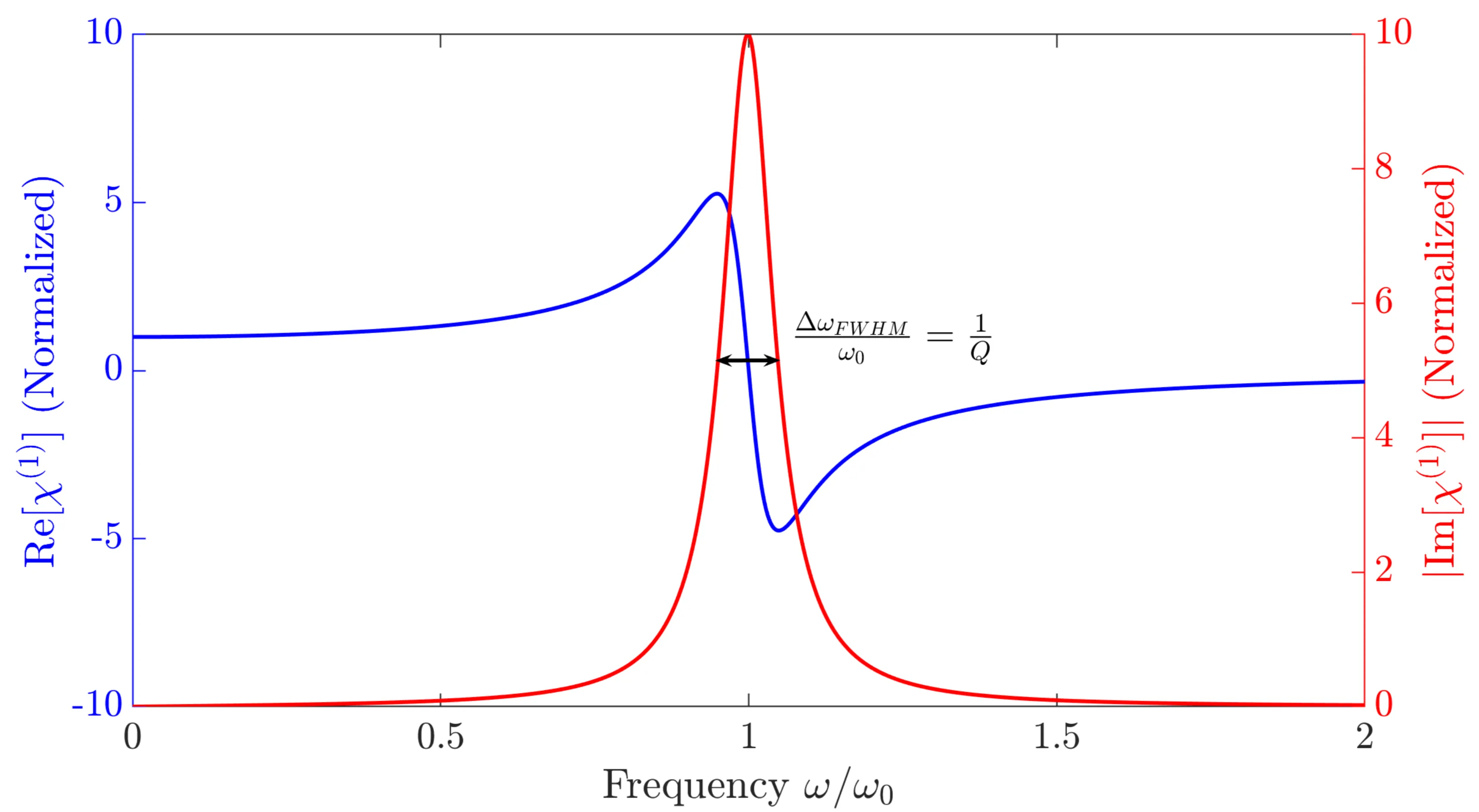
The real and imaginary parts of ${\chi }_e(\omega )={\chi }_e^{\prime }(\omega )+i{\chi }_e^{″}(\omega )$ are:

Both functions are plotted in the next figure, assuming weak damping ($\gamma \ll {\omega }_0$):

For high frequencies ($\omega \gg {\omega }_0$), the susceptibility ${\chi }_e^{\prime }(\omega )$ becomes small and negative, approaching zero, while ${\chi }_e^{″}(\omega )$ also approaches zero. The polarisation is out of phase with the electric field by nearly $\pi$ if ${\chi }_e^{\prime }<0$.
At resonance ($\omega ={\omega }_0$), the real part ${\chi }_e^{\prime }({\omega }_0)=0$, and the susceptibility is purely imaginary: ${\chi }_e({\omega }_0)=-i{\chi }_0\frac{{\omega }_0}{\gamma }$ from the original formula or $i{\chi }_0\frac{{\omega }_0}{\gamma }$ with the sign correction for ${\chi }_e^{″}$. If ${\chi }_e^{″}>0$, then ${\chi }_e({\omega }_0)=i{\chi }_0\frac{{\omega }_0}{\gamma }$. The polarisation is phase-shifted by $\pi /2$ relative to the electric field. The peak magnitude of ${\chi }_e^{″}({\omega }_0)$ is $Q{\chi }_0$, where $Q={\omega }_0/\gamma$ is the quality factor of the resonator. It quantifies how much energy is stored in the resonator compared to the energy lost per oscillation cycle. Reducing the damping $\gamma$ makes the resonance peak narrower and higher.
The same general arguments apply to magnetisation density, but at optical frequencies, magnetic resonances (${\chi }_m(\omega )$) are often negligible for most materials.

Very often, real systems can be represented as collections of resonators with a distribution of resonance frequencies ${\omega }_0^{(j)}$ and damping factors ${\gamma }^{(j)}$:

These different resonances can arise from different electronic transitions, vibrational modes, and so on.

2.1.2 Drude Model

A simplification of the Drude-Lorentz model for free charge carriers (like conduction electrons in a metal) is the Drude model. In this model, the electrons experience no restoring spring force, so the resonance frequency is ${\omega }_0=0$. The equation of motion becomes:

where we have replaced the damping rate with a collision (or scattering) rate $\gamma$. Assuming $E(t)=E_0{e}^{i\omega t}$, the steady-state solution for $x(t)=x_0{e}^{i\omega t}$ is:

With $P(t)=-Nex(t)$, we obtain $P(\omega )=-Ne{x}_0=\frac{N{e}^2/m_e}{{\omega }^2-i\gamma \omega }E(\omega )$.
The susceptibility ${\chi }_e(\omega )=P(\omega )/({\epsilon }_{0}E(\omega ))$ is then:

where ${\omega }_p=\sqrt{N{e}^2/(m_e{\epsilon }_0)}$ is the plasma frequency, and $N$ is the free carrier concentration.
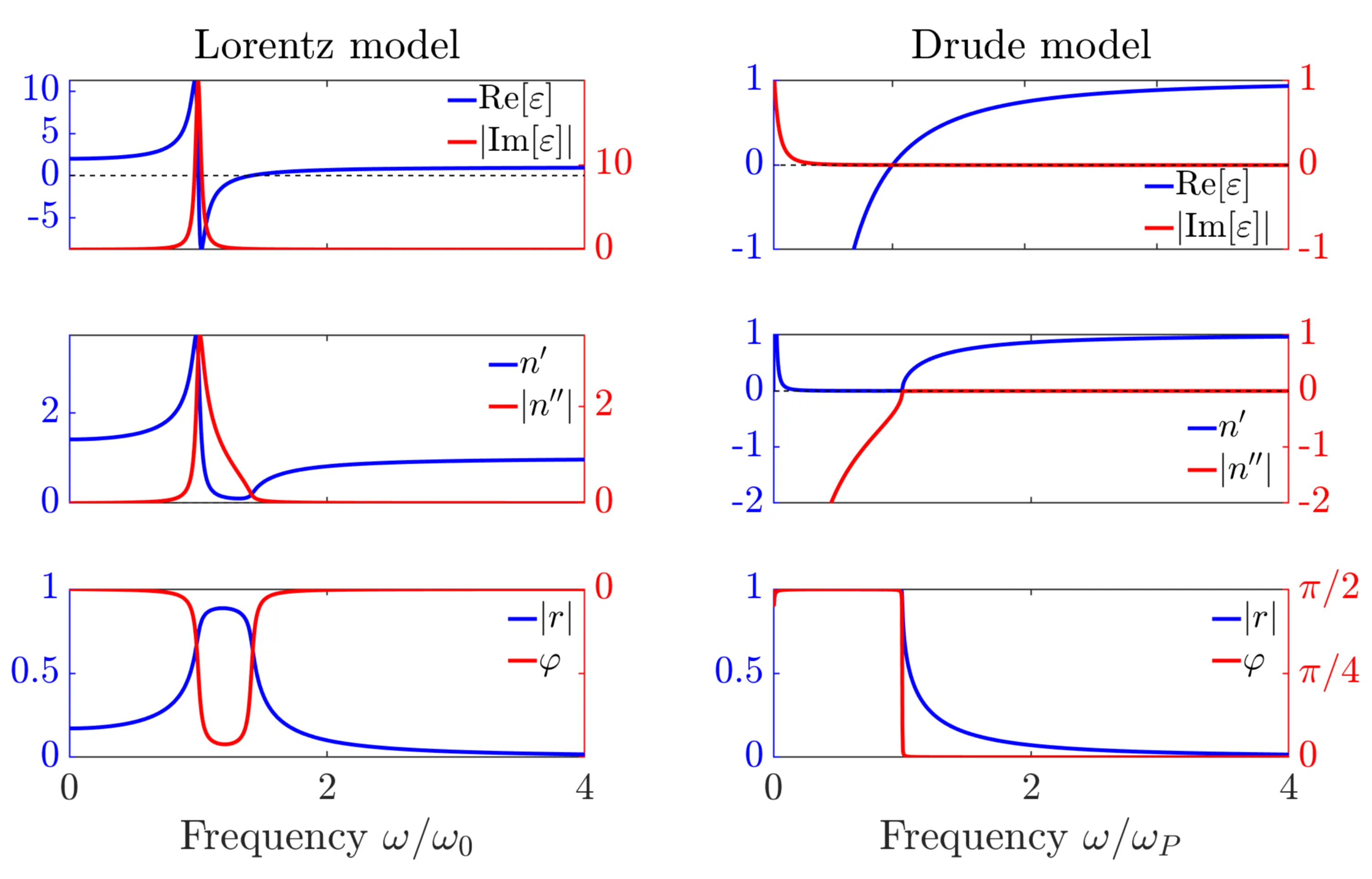
The real and imaginary parts are:

In the high-frequency limit where $\omega \gg \gamma$ (low damping), the susceptibility is predominantly real, and the relative permittivity ${\epsilon }_r(\omega )=1+{\chi }_e(\omega )$ becomes:

This is the dispersion relation for an undamped plasma, and we differentiate between different cases:

• For frequencies below the plasma frequency ($\omega <{\omega }_p$), we have ${\epsilon }_r(\omega )<0$. The refractive index $n=\sqrt{{\epsilon }_r}$ is imaginary, so the wavevector $k=n\omega /c$ is imaginary. The wave does not propagate but is attenuated (evanescent) within the metal. Metals are highly reflective.
• For frequencies above the plasma frequency ($\omega >{\omega }_p$), we have $0<{\epsilon }_r(\omega )<1$. Both $n$ and $k$ are real. The wave propagates. The metal becomes transparent.
• For $\omega ={\omega }_p$, we have ${\epsilon }_r({\omega }_p)=0$. In this idealised case, $n=0$, $k=0$. This frequency marks the onset of propagation of transverse waves. Longitudinal plasma oscillations (volume plasmons) occur at ${\omega }_p$ where ${\epsilon }_r({\omega }_p)=0$.

Next, let us compare both the Drude-Lorentz and Drude model for the reflectivity $R=|r{|}^2$, where

is the Fresnel reflection coefficient for normal incidence from vacuum onto a medium with complex refractive index $\tilde{n}=n^{\prime }+i{n}^{″}$.

To model silver, the fit is usually done using a combination:

where the Drude part accounts for free electrons and Lorentz oscillators account for interband transitions. The Drude model alone is often a good fit for the low frequency (infrared) region. However, at higher frequencies (visible/UV), contributions from Lorentz oscillators representing interband transitions must be taken into account.

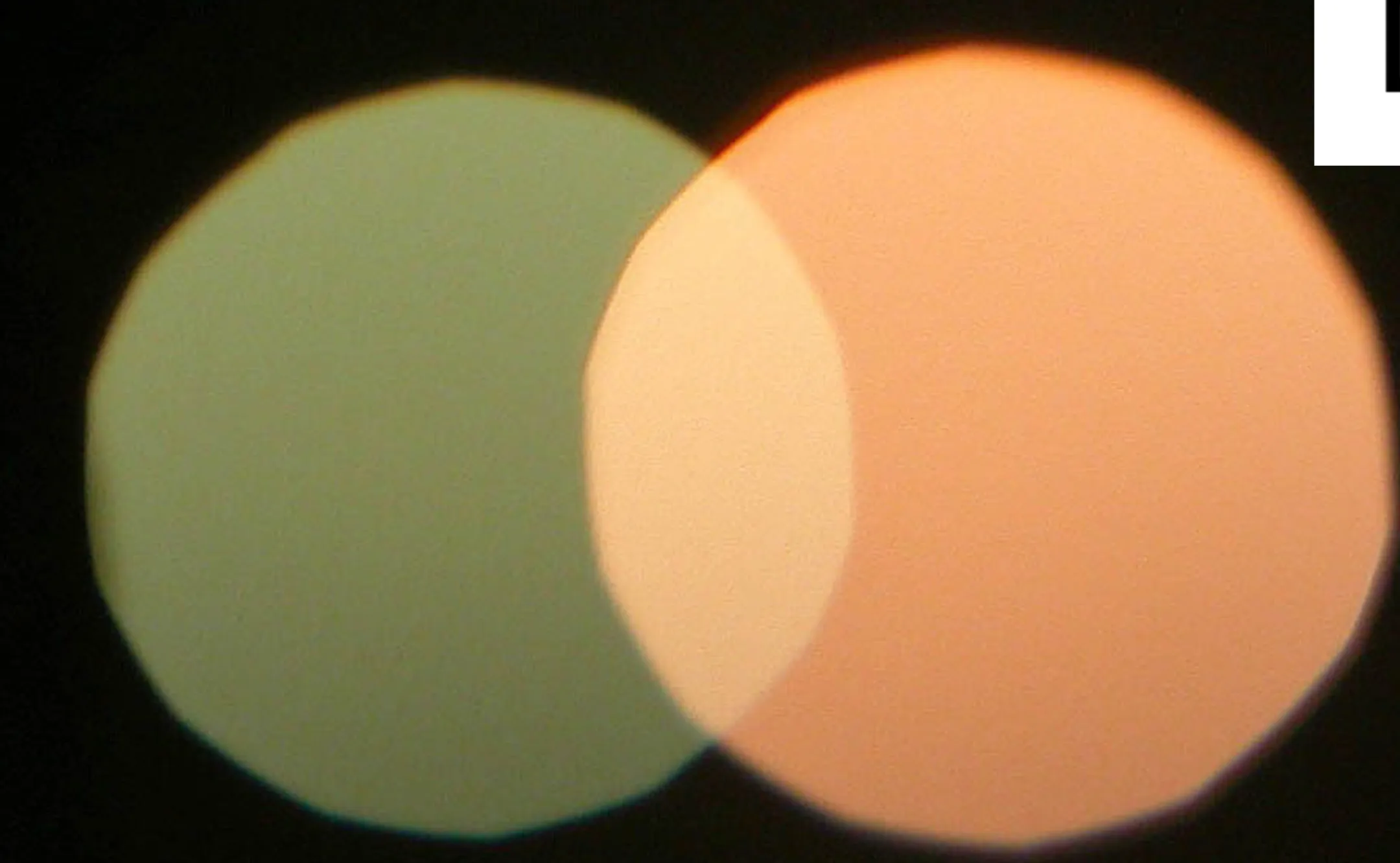
Lastly, let us discuss a simple implication of the plasma frequency. Consider gold, which has high reflectivity for wavelengths above approximately $500-600\text{nm}$ (red/yellow light) but lower reflectivity (and increased absorption) for shorter wavelengths (green/blue light). This results in reflected white light appearing yellowish/golden, while transmitted light through a very thin gold film can appear bluish-green. This behaviour is related to its plasma frequency and interband transitions. For a thin film of gold, while some absorption occurs, the relation $A+R+T=1$ (Absorbance + Reflectance + Transmittance) holds.

In this framework, the colour of metals can be understood by considering the effect of both the plasma frequency (Drude response) and interband transitions (Lorentz oscillators) on the spectral reflectivity.

2.2 Kramers-Kronig Relations

From the previous section, we have seen that the frequency dependence of the refractive index (dispersion, related to ${\chi }_e^{\prime }$) and absorption (related to ${\chi }_e^{″}$) are interconnected. A dispersive material must be absorptive over some frequency range, and must exhibit a frequency-dependent absorption coefficient if it is dispersive. This general principle is mathematically captured by the Kramers-Kronig relations. Even with our very simplistic models for susceptibility, linear response theory has important implications regarding causality.

The Kramers-Kronig relations connect the real and imaginary parts of a complex response function, such as the electric susceptibility ${\chi }_e(\omega )$. They are a direct mathematical consequence of causality (the response cannot precede the stimulus) and the assumption that the response function ${\chi }_e(t)$ is real.
The relations are:

$\mathcal{P}$ denotes the Cauchy Principal Value of the integral. The response function ${\chi }_e(t)$ being real ensures ${\chi }_e(\omega )={\chi }_e^{\ast }(-\omega )$, leading to ${\chi }_e^{\prime }(\omega )$ being even and ${\chi }_e^{″}(\omega )$ being odd, allowing the integrals to be written over $[0,\mathrm{\infty })$.
These relations are powerful: they allow the calculation of one part of the complex susceptibility (or permittivity, or refractive index) if the other part is known over the entire frequency spectrum. Practically, measuring over all frequencies is impossible, but measurements over a broad range combined with physically reasonable extrapolations or models for regions far from resonances can be used. For instance, measuring the absorption spectrum ($\sim {\chi }_e^{″}(\omega )$) over a wide range allows the calculation of the refractive index dispersion ($\sim {\chi }_e^{\prime }(\omega )$).

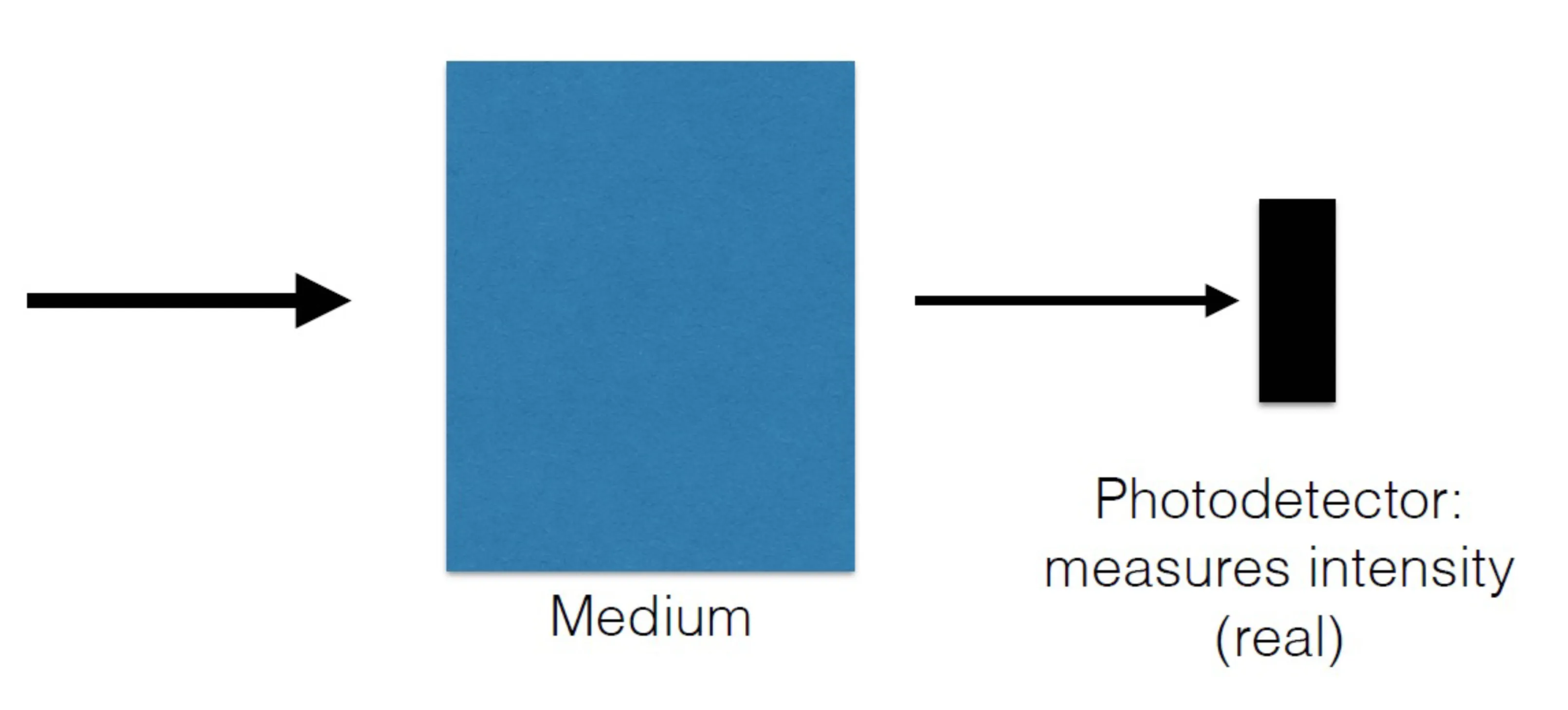
Consider sending light through a medium and detecting the transmitted intensity with a photodetector:

If the goal is to determine the complex susceptibility ${\chi }_e(\omega )$, one typically needs to measure both amplitude and phase changes upon interaction with the medium. A simple photodetector measures intensity, thereby losing phase information which is crucial for the real part of the refractive index (and thus ${\chi }_e^{\prime }$). However, by carefully measuring the absorption spectrum (related to ${\chi }_e^{″}$) as a function of frequency, the Kramers-Kronig relations can be used to reconstruct the dispersive part ${\chi }_e^{\prime }$ (and thus the full complex refractive index).

2.3 Equations in Frequency Domain

Consider again the macroscopic field relations in the time domain:

Assuming linear responses $\mathbf{P}(t)={\epsilon }_0({\chi }_e\ast \mathbf{E})(t)$ and $\mathbf{M}(t)=({\chi }_m\ast \mathbf{H})(t)$, Fourier transforming these equations (convolution becomes multiplication) results in:

Here, ${\epsilon }_r(\omega )=1+{\chi }_e(\omega )$ is the complex relative permittivity (or dielectric function), and ${\mu }_r(\omega )=1+{\chi }_m(\omega )$ is the complex relative permeability. $\epsilon (\omega )={\epsilon }_0{\epsilon }_r(\omega )$ and $\mu (\omega )={\mu }_0{\mu }_r(\omega )$ are the absolute complex permittivity and permeability, respectively.
Next, let us transform Maxwell's equations to frequency space. Using the Fourier transform property that $\frac{\partial }{\partial t}\leftrightarrow i\omega$:
For no free charges (${\rho }_f=0$) and no free currents (${\mathbf{j}}_f=0$), we find:

It should be noted here that a truly non-dispersive medium has an instantaneous response. If ${\chi }_e(\omega )={\hat{\chi }}_e$ (a constant independent of frequency), then its inverse Fourier transform is:

This means $\mathbf{P}(t)={\epsilon }_0{\hat{\chi }}_e\mathbf{E}(t)$, an instantaneous relation.

2.4 Helmholtz Equation

Let us start from Faraday's law in the frequency domain, $\mathrm{\nabla }\times \mathbf{E}(\mathbf{r},\omega )=-i\omega \mathbf{B}(\mathbf{r},\omega )$, and apply the curl operator:

Using the vector identity $\mathrm{\nabla }\times (\mathrm{\nabla }\times \mathbf{A})=\mathrm{\nabla }(\mathrm{\nabla }\cdot \mathbf{A})-{\mathrm{\nabla }}^2\mathbf{A}$, and assuming a homogeneous medium where $\mathrm{\nabla }\cdot \mathbf{E}=0$ (which follows from $\mathrm{\nabla }\cdot \mathbf{D}=0$ if ${\epsilon }_r$ is spatially constant and ${\rho }_f=0$), the left side becomes $-{\mathrm{\nabla }}^2\mathbf{E}$.
For the right side, substitute $\mathbf{B}={\mu }_0{\mu }_r(\omega )\mathbf{H}$ and then Ampère-Maxwell's law $\mathrm{\nabla }\times \mathbf{H}=i\omega \mathbf{D}$ (for ${\mathbf{j}}_f=0$):

Substitute $\mathbf{D}={\epsilon }_0{\epsilon }_r(\omega )\mathbf{E}$:

Rearranging gives the Helmholtz equation:

Using $c^2=1/({\mu }_0{\epsilon }_0)$ and defining the complex refractive index $n(\omega )=\sqrt{{\mu }_r(\omega ){\epsilon }_r(\omega )}$, this becomes:

This is the wave equation in the frequency domain for a linear, homogeneous, isotropic medium.
We can write $n(\omega )=n^{\prime }(\omega )+i{n}^{″}(\omega )$. This makes the wavevector $\mathbf{k}(\omega )$ complex. For a plane wave propagating in the $\mathbf{r}$-direction, $\mathbf{k}(\omega )=k(\omega )\hat{\mathbf{r}}=n(\omega )\frac{\omega }{c}\hat{\mathbf{r}}$.
The Fourier transform of a monochromatic plane wave $E(t)={\tilde{E}}_0{e}^{i({\omega }_{1}t-\mathbf{k}({\omega }_1)\cdot \mathbf{r})}$ is $E(\omega )=2\pi {\tilde{E}}_0\delta (\omega -{\omega }_1)e^{-i\mathbf{k}({\omega }_1)\cdot \mathbf{r}}$. A general solution can be built from these.
For a specific frequency $\omega$, a plane wave solution is $\mathbf{E}(\mathbf{r},t)={\tilde{\mathbf{E}}}_0{e}^{i(\mathbf{k}(\omega )\cdot \mathbf{r}-\omega t)}$.
Let $\mathbf{k}(\omega )={\mathbf{k}}^{\prime }(\omega )+i{\mathbf{k}}^{″}(\omega )$. Then the spatial part is $e^{i{\mathbf{k}}^{\prime }(\omega )\cdot \mathbf{r}}{e}^{-{\mathbf{k}}^{″}(\omega )\cdot \mathbf{r}}$.
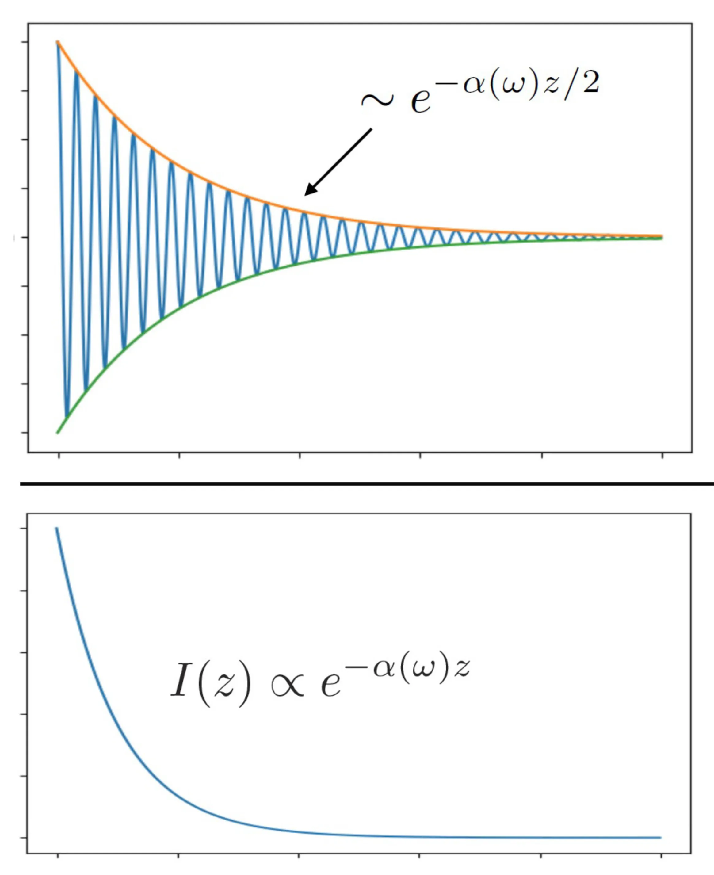
The term $e^{i{\mathbf{k}}^{\prime }(\omega )\cdot \mathbf{r}}$ represents the oscillating phase, while $e^{-{\mathbf{k}}^{″}(\omega )\cdot \mathbf{r}}$ represents an exponential decay of the wave amplitude if ${\mathbf{k}}^{″}(\omega )$ is positive and points in the direction of propagation $\mathbf{r}$. This decay causes a loss of energy carried by the wave as it moves through the medium.
The imaginary part of the refractive index, $n^{″}(\omega )$, determines ${\mathbf{k}}^{″}(\omega )$. For a passive, lossy medium, $n^{″}(\omega )>0$ (by common convention). If so, ${\mathbf{k}}^{\prime }(\omega )$ and ${\mathbf{k}}^{″}(\omega )$ are parallel.
The wavelength in the medium is defined by the real part of the wavevector: ${\lambda }_n=\frac{2\pi }{|{\mathbf{k}}^{\prime }(\omega )|}$.
The phase velocity is given by $v_p(\omega )=\frac{\omega }{|{\mathbf{k}}^{\prime }(\omega )|}=\frac{c}{n^{\prime }(\omega )}$. It describes the speed at which surfaces of constant phase propagate.
The time-averaged intensity of the wave is related to $|{\tilde{\mathbf{E}}}_0{|}^2{e}^{-2{\mathbf{k}}^{″}(\omega )\cdot \mathbf{r}}$. We define the intensity absorption coefficient as $\alpha (\omega )=2|{\mathbf{k}}^{″}(\omega )|=2n^{″}(\omega )\omega /c$. The intensity then decays as $I(z)=I_0{e}^{-\alpha (\omega )z}$ (if propagating in $z$-direction). This is illustrated next:

2.5 Refractive Index in Dispersive Media

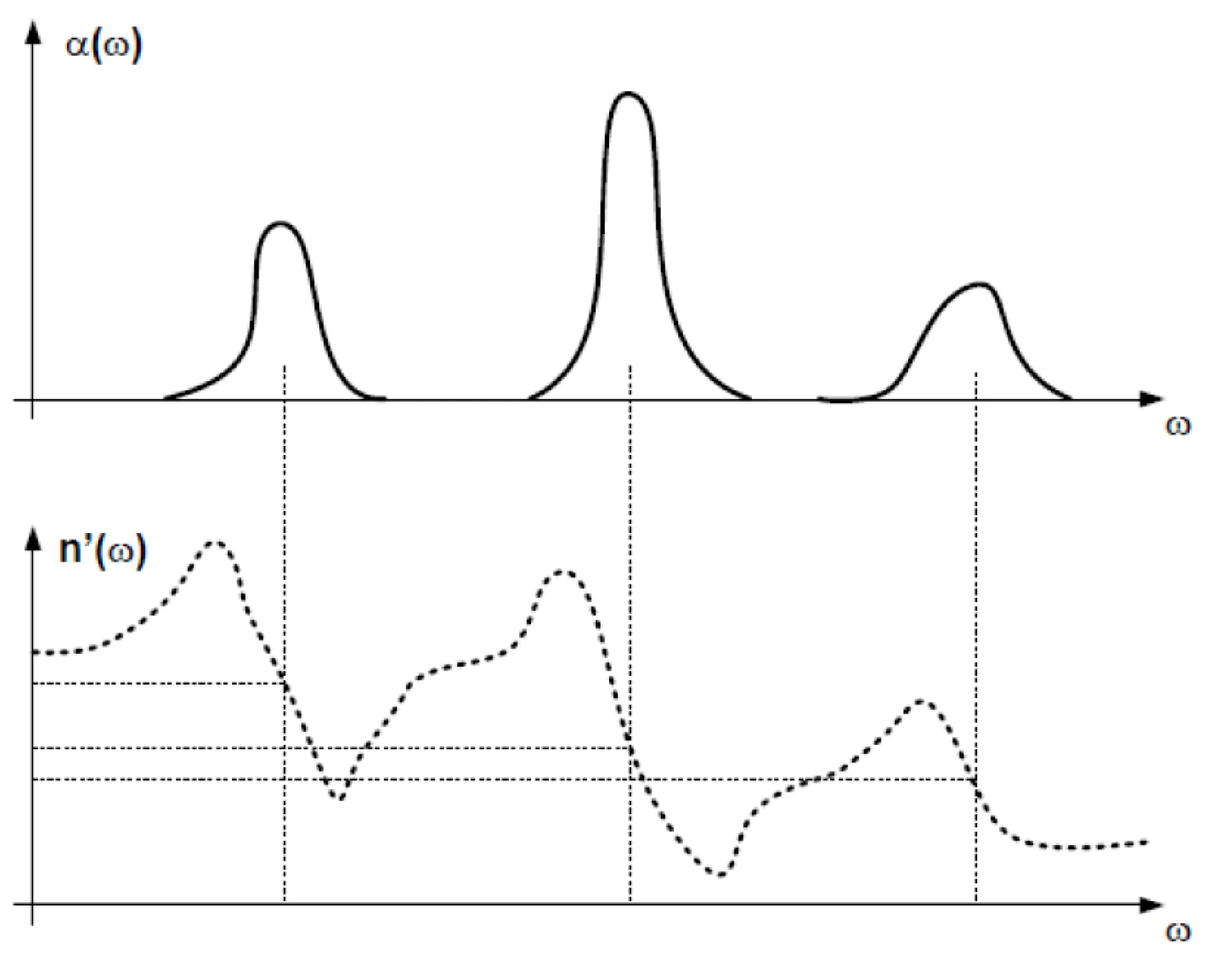
Again, let us stress that the frequency-dependence of the real part of the refractive index $n^{\prime }(\omega )$ (dispersion) is inherently related via the Kramers-Kronig relations to the frequency-dependence of its imaginary part $n^{″}(\omega )$ (absorption). If there is absorption ($n^{″}(\omega )\ne 0$) at some frequencies, the refractive index $n^{\prime }(\omega )$ must be dispersive (frequency-dependent) over all frequencies, and vice-versa. While absorption resonances ($\text{peaks in }{n}^{″}(\omega )$) are often localised in frequency, the associated changes in the refractive index $n^{\prime }(\omega )$ extend over a much broader frequency range. We have seen: If there is absorption anywhere in the spectrum, the refractive index $n^{\prime }(\omega )$ becomes dispersive everywhere. This is shown in the next figure for a material with three distinct absorption resonances:

For most optically transparent media (meaning they have low absorption in the visible range), the strongest electronic absorption resonances (corresponding to ${\omega }_0$ in the Lorentz model) typically lie in the ultraviolet. For frequencies $\omega$ in the visible range, we are often in the regime $\omega \ll {\omega }_0$. Assuming weak damping ($\gamma \ll {\omega }_0$), the imaginary part of the susceptibility ${\chi }_e^{″}(\omega )$ (and thus $n^{″}(\omega )$) becomes very small in this transparent region, while its real part ${\chi }_e^{\prime }(\omega )$ typically increases with $\omega$. Since $n^{\prime }(\omega )\approx \sqrt{1+{\chi }_e^{\prime }(\omega )}$ (for ${\chi }_e^{\prime }$ small or $(n^{\prime }{)}^2\approx 1+{\chi }_e^{\prime }$), this implies that the refractive index exhibits 'normal' dispersion:

Near an absorption resonance ($\omega \approx {\omega }_0$), the dispersion typically becomes anomalous before returning to normal at higher frequencies above the resonance.
In practice, empirical interpolation formulas are used to describe $n^{\prime }(\omega )$ (or $n^{\prime }({\lambda }_0)$) in regions of transparency. The imaginary part is often ignored if absorption is small. The most well-known of these formulas is the Sellmeier equation:

where the vacuum wavelength ${\lambda }_0=c/f$ is often expressed in micrometres. Usually, two or three terms in the sum are sufficient to fit experimental data for many glasses over the visible and near-infrared. The similarity of the Sellmeier equation to a sum of Lorentz oscillators arises because it can be derived assuming resonances are very narrow (like delta functions in ${\chi }_e^{″}(\omega )$), which is a good approximation far from these resonances. The coefficients $B_j$ are related to the strength of the $j$-th resonance, and $C_j={\lambda }_{0,j}^2$ where ${\lambda }_{0,j}$ is the resonance wavelength of the $j$-th oscillator.

Lastly, note that the Sellmeier equation typically lacks accuracy in the XUV (extreme ultraviolet) and X-ray range (short wavelengths), where the refractive index of any material is very close to 1. These small deviations from unity are often described using $n(\omega )=1-\delta (\omega )+i{\beta }_{\text{abs}}(\omega )$ (here ${\beta }_{\text{abs}}$ is the absorption index, not propagation constant). Both $\delta$ and ${\beta }_{\text{abs}}$ are usually small and positive for ${\lambda }_0\sim 0.1\text{nm}$ to $100\text{nm}$, unless the frequency is very close to an atomic absorption edge (which corresponds to an ionisation threshold or inner-shell transition).

2.6 Light Pulses

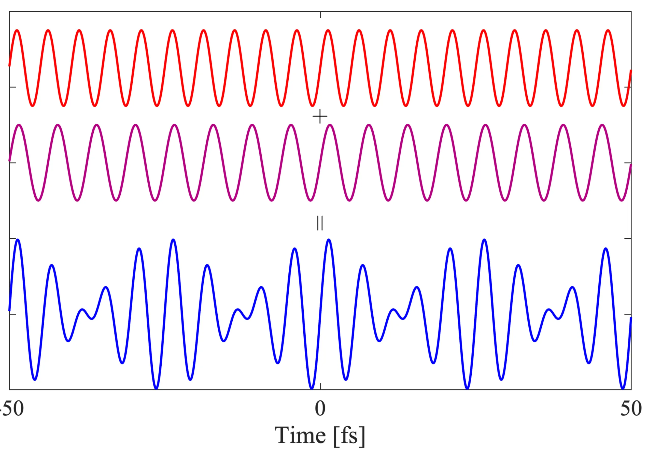
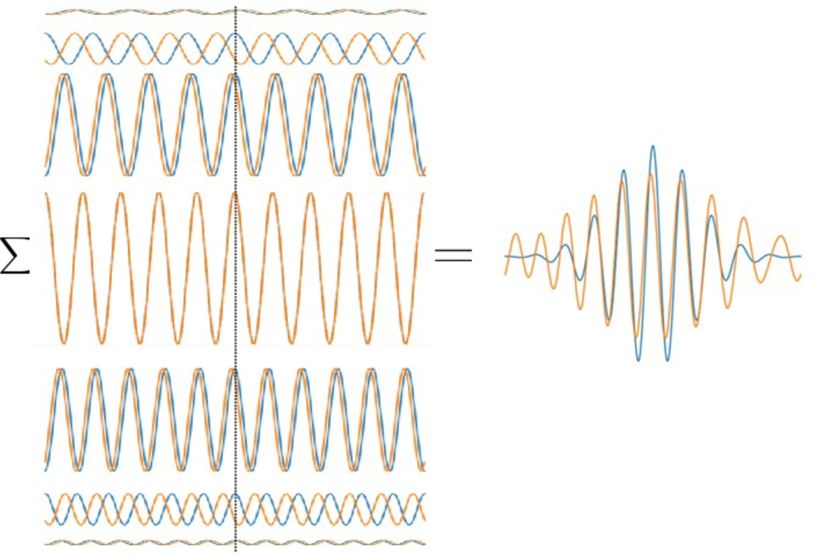
Let us consider an important example of a non-monochromatic wave: a light pulse. Light pulses, as opposed to continuous monochromatic plane waves, are finite in time duration and thus also have a finite spatial extent along the propagation direction. Here, we still treat them as infinitely extended transverse to the propagation direction, so as plane wave pulses. It is understood that a pulse can be represented as a superposition of plane waves of varying wavelengths or frequencies:

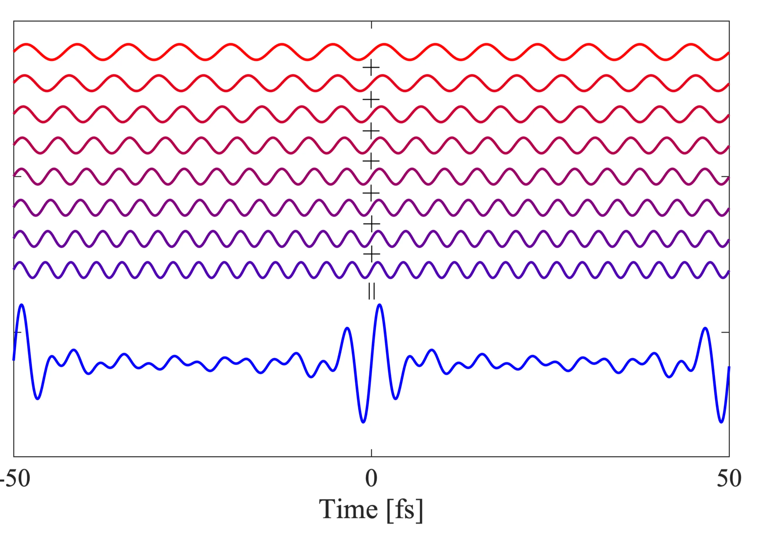
In this conceptual image, a 'red' (lower frequency) and a 'violet' (higher frequency) wave are superposed to get the resultant 'blue' wave (the pulse envelope). The colours are illustrative and not necessarily related to physical colours. It turns out that the more frequency components (waves with different frequencies) are added coherently, the 'narrower' in time the resulting pulse can become:

The general effect of superimposing multiple waves with frequencies ${\omega }_m={\omega }_a+m\mathrm{\Delta }\omega$ (where $m$ is an integer) is to produce constructive interference at times $t_p=p\cdot 2\pi /\mathrm{\Delta }\omega$ (where $p$ is an integer) and destructive interference elsewhere, leading to a train of pulses. If many waves with a broad spectrum around a centre frequency ${\omega }_a$ are superposed, and if $\mathrm{\Delta }\omega$ represents the approximate overall bandwidth, then a short pulse of duration $\sim 1/\mathrm{\Delta }\omega$ can be formed.

Constructive interference of two waves
Let us take a step back and consider the superposition of two plane waves with real amplitudes ${\mathbf{E}}_0$, frequencies ${\omega }_1$ and ${\omega }_2$, and corresponding wavevectors $\mathbf{k}({\omega }_1)$ and $\mathbf{k}({\omega }_2).$ Assume they are in phase at $\mathbf{r}=0,t=0$.

Let ${\omega }_a=({\omega }_1+{\omega }_2)/2$ be the average (carrier) frequency and $\mathrm{\Delta }\omega =({\omega }_2-{\omega }_1)$ be the frequency difference. Similarly, let ${\mathbf{k}}_a=(\mathbf{k}({\omega }_1)+\mathbf{k}({\omega }_2))/2$ and $\mathrm{\Delta }\mathbf{k}=(\mathbf{k}({\omega }_2)-\mathbf{k}({\omega }_1))$.
The superposition $\mathbf{E}(t)={\mathbf{E}}_1(t)+{\mathbf{E}}_2(t)$ at $\mathbf{r}=0$ can be rewritten using trigonometric identities as:

This represents a fast oscillation at ${\omega }_a$ modulated by a slower envelope oscillating at $\mathrm{\Delta }\omega /2$.
To find the speed of this envelope maximum (a point of constructive interference), consider the condition that the phases of the two waves remain equal as the wave propagates a distance $\mathrm{\Delta }z$ in time $\mathrm{\Delta }t$ (assuming 1D propagation along $z$, so $k=k_z$):

This leads to $\mathrm{\Delta }z(\mathrm{\Delta }{k}^{\prime })=\mathrm{\Delta }t(\mathrm{\Delta }\omega )$, where $\mathrm{\Delta }{k}^{\prime }=k^{\prime }({\omega }_2)-k^{\prime }({\omega }_1)$.
The velocity of this constant-phase point of the envelope is the group velocity $v_g$:

In the limit of a small frequency difference ($\mathrm{\Delta }\omega \to 0$), we obtain the group velocity as:

Using $k^{\prime }(\omega )=n^{\prime }(\omega )\omega /c$, we can express $v_g$ as:

Sometimes, the group index $n_g$ is used, defined as:

The group velocity represents the speed of the pulse envelope if the envelope changes slowly and the spectral bandwidth is narrow enough that $v_g$ is approximately constant over that bandwidth. Deviations from this ideal condition lead to pulse broadening and distortion, known as group velocity dispersion (GVD). For transparent optical materials away from resonances, the group velocity is usually smaller than the phase velocity $v_p=c/n^{\prime }$.

Lastly, consider the following figure illustrating phase and group velocities:

In this animation, the green points represent points moving at the group velocity (envelope speed), while red points represent points moving at the phase velocity (carrier wave speed). The figure illustrates how these two velocities can differ in a dispersive medium.

2.7 Time-Bandwidth Product of Wavepackets

A light pulse is formed by superimposing plane waves with different frequencies. In a continuous form, this superposition is described by the inverse Fourier transform:

We generally call $\mathbf{E}(\omega )$ the spectrum of the pulse, indicating the complex amplitude (magnitude and phase) of each monochromatic constituent of the pulse. The spread of frequencies in the spectrum is its bandwidth $\mathrm{\Delta }\omega$ (or $\mathrm{\Delta }f=\mathrm{\Delta }\omega /2\pi$), which is usually much smaller than the average/centre frequency ${\omega }_a$ of the pulse for well-defined pulses. The spectral energy density is proportional to $|\mathbf{E}(\omega ){|}^2$.

The electric field as a function of frequency, $\mathbf{E}(\omega )$, and the electric field as a function of time, $\mathbf{E}(t)$, are Fourier transform pairs. This mathematical relationship has an important implication: there is a fundamental limit to how short a pulse duration $\mathrm{\Delta }t$ can be for a given spectral bandwidth $\mathrm{\Delta }\omega$. This is quantified by the time-bandwidth product (TBP).
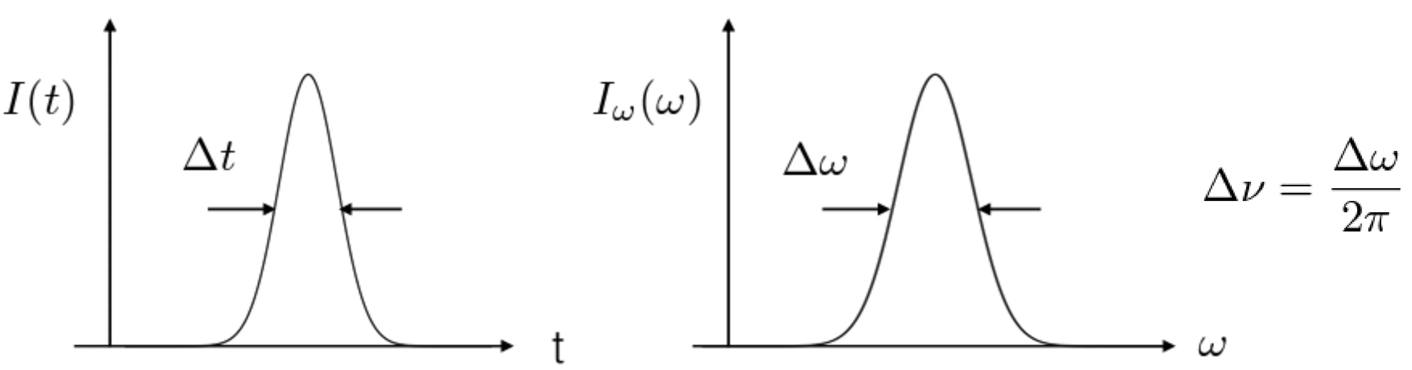
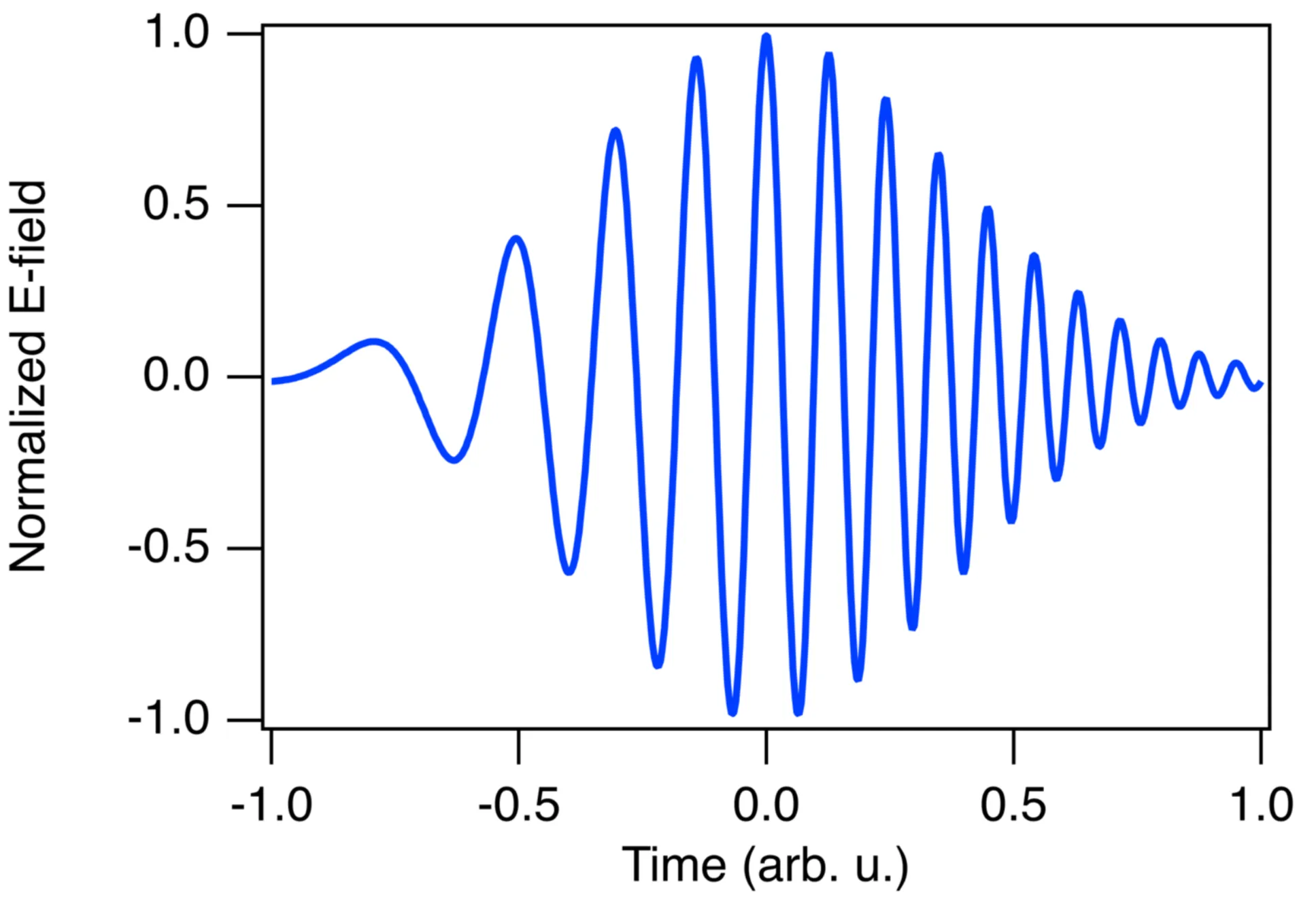
Consider the next figure, showing the intensity profile in time, $|E(t){|}^2$, and the spectral intensity, $|E(\omega ){|}^2$:

The Fourier transform uncertainty principle states that the product $\mathrm{\Delta }t\cdot \mathrm{\Delta }\omega$ (or $\mathrm{\Delta }t\cdot \mathrm{\Delta }f$) has a minimum possible value, which depends on the pulse shape (definitions of $\mathrm{\Delta }t$ and $\mathrm{\Delta }\omega$, such as Full Width at Half Maximum, also affect this value). We call this product the time-bandwidth product. Pulses that achieve this minimum are called transform-limited pulses. For such pulses, the spectral phase $\arg [\mathbf{E}(\omega )]$ is constant or, at most, linear in frequency across the pulse bandwidth.

Pulses that are not transform-limited possess a non-linear spectral phase. This results in a pulse duration $\mathrm{\Delta }t$ that is longer than the minimum allowed by its spectral bandwidth. These pulses have a time-dependent instantaneous oscillation frequency, a phenomenon known as chirp. If $\phi (t)$ is the total phase of the complex analytic signal associated with $\mathbf{E}(t)$, the instantaneous frequency is $\omega (t)=\frac{d\phi (t)}{dt}$. A chirp means $\omega (t)$ is not constant.

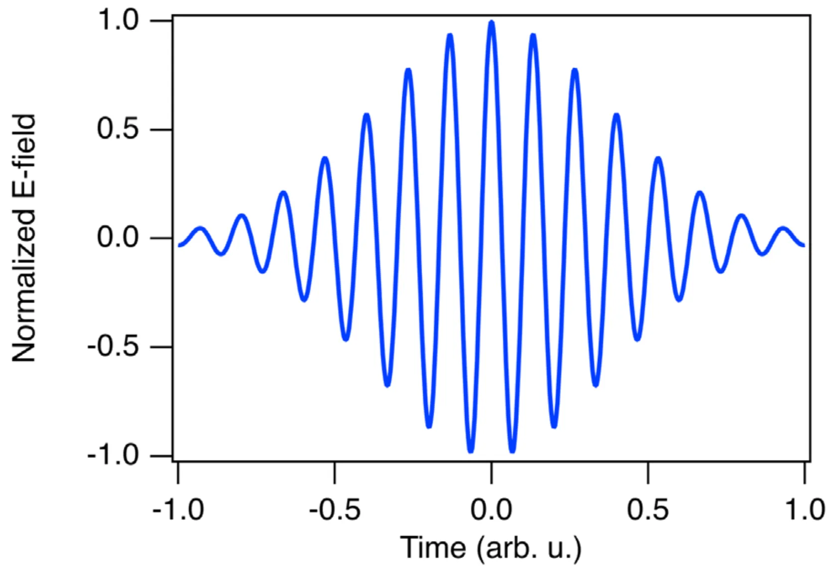
Consider a transform-limited (therefore unchirped) Gaussian pulse:

The next figure shows a chirped Gaussian pulse. By definition, its time-bandwidth product is greater than the minimum possible for a Gaussian shape: $\mathrm{\Delta }t\cdot \mathrm{\Delta }\nu >{\text{TBP}}_{\text{Gaussian}}$.

To illustrate the effect of a chirp, consider the difference between an unchirped (blue) and a chirped (orange) light pulse, both having the same spectral amplitude magnitude:

We can see that the pulse duration (FWHM) of the unchirped blue pulse is shorter than that of the chirped orange pulse. If a chirp is positive (up-chirp), lower frequencies precede higher frequencies in time. If a chirp is negative (down-chirp), higher frequencies precede lower frequencies. The type of chirp acquired by a pulse propagating through a dispersive medium depends on the sign of the group velocity dispersion (GVD) of the medium.
Usually, GVD is quantified by the dispersion parameter $D_{\lambda }$:

with its units typically being ps/(nm$\cdot$km) in telecommunications, where optical fibres can be kilometres long. The duration ${\tau }_p(\mathrm{\Delta }z)$ of an initially transform-limited Gaussian pulse with duration $\mathrm{\Delta }{t}_0$ (FWHM) after propagating a distance $\mathrm{\Delta }z$ through a medium with dispersion $D_{\lambda }$ and initial spectral width $\mathrm{\Delta }{\lambda }_0$ can be approximated by:

This shows pulse broadening due to dispersion.

2.8 Phase, Group and Front Velocity

It is known that the phase velocity $v_p=c/n^{\prime }(\omega )$ can exceed the speed of light in vacuum $c$ (for $n^{\prime }(\omega )<1$), particularly for XUV light in materials or near absorption resonances in any spectral range. The group velocity $v_g=c/n_g(\omega )$ can also exceed $c$ (if $n_g(\omega )<1$) or even become negative near a strong absorption line where $d{n}^{\prime }/d\omega$ can be large and negative. However, these phenomena do not violate the principles of relativity, which state that no energy or information can be transmitted faster than $c$.

Neither the phase velocity nor the group velocity are, in general, reliable measures for the speed of information transmission. The phase velocity describes the velocity of points of constant phase (such as wave crests or zero-crossings). Since a monochromatic wave extends infinitely in time and space, observing one zero-crossing allows prediction of all others, so no new information is conveyed by its propagation at $v_p$. The group velocity describes the velocity of the peak of the pulse envelope under certain conditions (narrow bandwidth, slowly varying envelope, negligible higher-order dispersion). However, for pulses with broad bandwidths or in regions of strong dispersion, the pulse shape can change dramatically, and the group velocity may not accurately represent the speed of any particular feature of the pulse, nor the speed of information. For analytic pulse shapes (whose future is determined by their past), the propagation of the envelope peak may not constitute signal transmission in the strictest sense.

The true maximum speed of information or energy transmission is the front velocity of a pulse, which is the speed of any non-analytic feature at the very beginning of a pulse (the wavefront). It has been shown that the front velocity is always equal to $c$ in vacuum, regardless of the medium the pulse subsequently enters, and it cannot exceed $c$ in any medium.