Jump back to chapter selection.
Table of Contents
10.1 Planar Mirror Waveguide
10.2 Planar Dielectric Waveguide
10.3 Optical Fibres
10 Waveguides
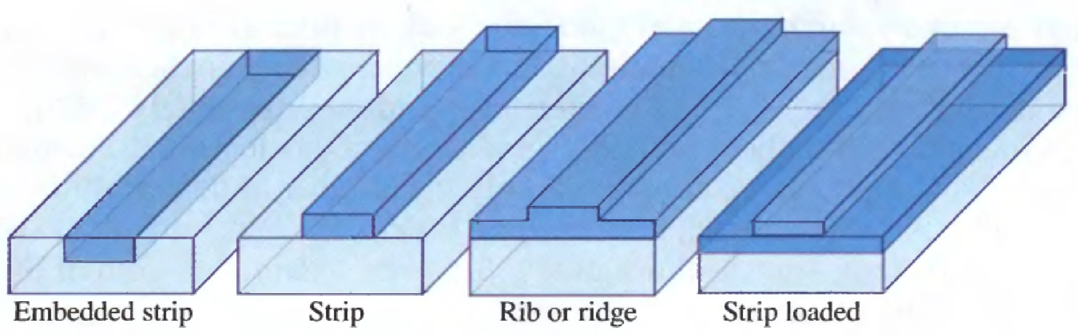
Waveguides are devices that transmit and guide light and other electromagnetic radiation along a prescribed path. In contrast to traditional free-space optics, this guidance occurs within or along a material structure. Waveguides offer the advantage of alignment robustness and, particularly in the case of optical fibres, the ability to circumvent obstructions. They are used extensively in telecommunication over long distances, and also in biomedical applications where light needs to be delivered to or collected from difficult-to-access places. Waveguides are key components of 'integrated optics'. They come in many different forms, as the following figure illustrates:
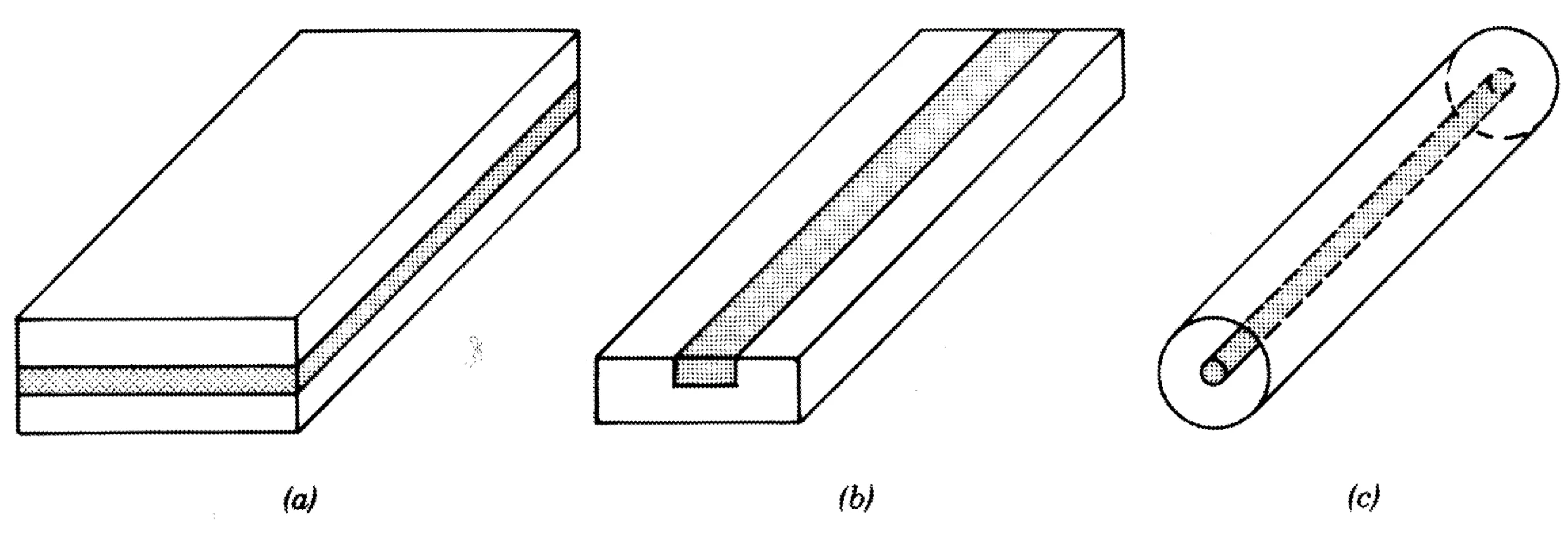
The difference between the colours in the schematic typically represents different refractive indices. The figure shows, from (a) to (c): a slab waveguide, a strip (or channel) waveguide, and an optical fibre.
10.1 Planar Mirror Waveguide
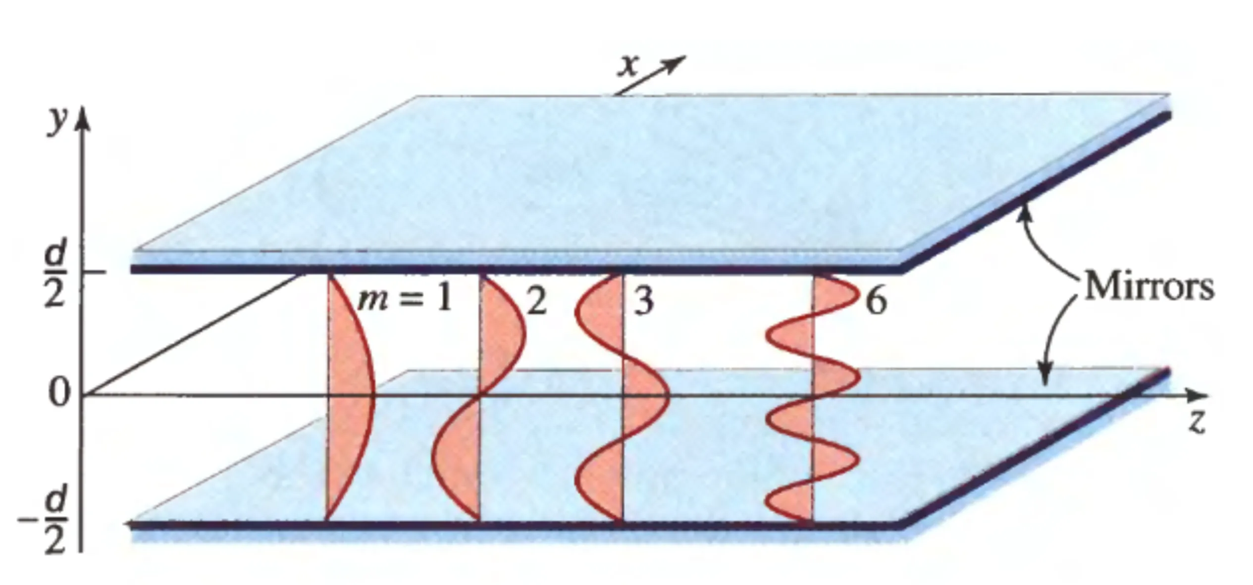
The following figure shows a planar mirror waveguide, consisting of two parallel, highly reflective (ideally perfect) mirrors placed a distance
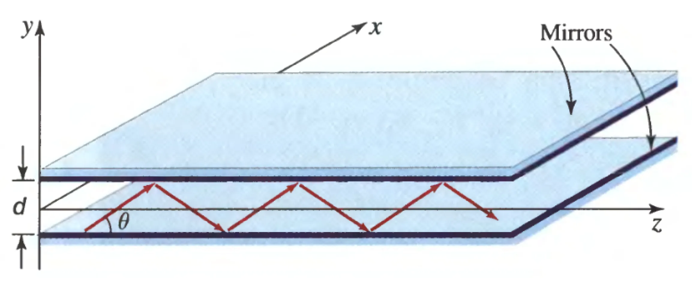
One way to treat electromagnetic radiation within this planar mirror waveguide is by using a ray optics picture. We can identify guided modes as those waves that self-consistently interfere (that is, constructively interfere) after undergoing reflections from each mirror. Consider a plane wave bouncing between the mirrors, making an angle
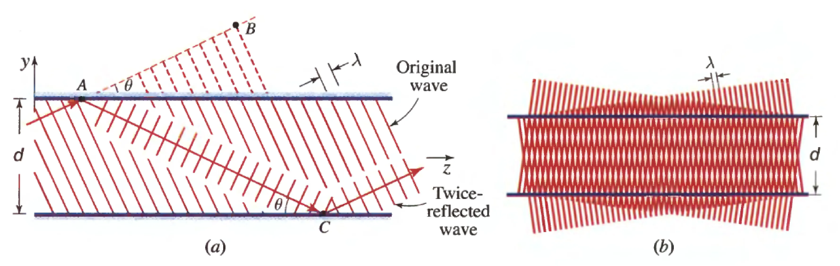
For constructive interference, the phase difference accumulated over one round trip in the transverse (
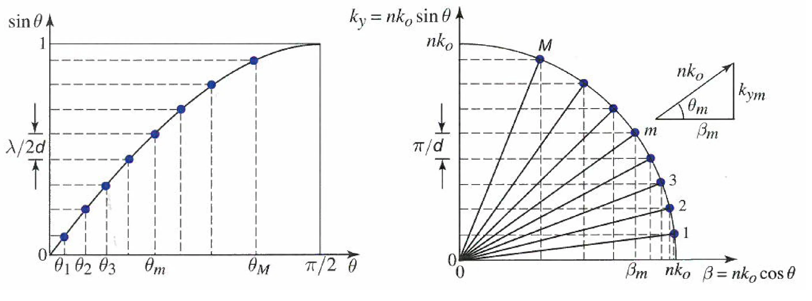
More directly, considering the transverse wavevector component
The wavevector components are
From
The propagation constant for mode
For
Modes of higher order
Alternatively, considering a superposition of two plane waves with wavevectors
Let
Boundary conditions
These require either
or
Combining these,
10.1.1 TE Modes
For Transverse Electric (TE) modes, the electric field is transverse to the direction of propagation
where
for (if boundaries at ) for odd (symmetric modes about , boundaries at ) for even (antisymmetric modes about , boundaries at )
Odd modes (
Even modes (
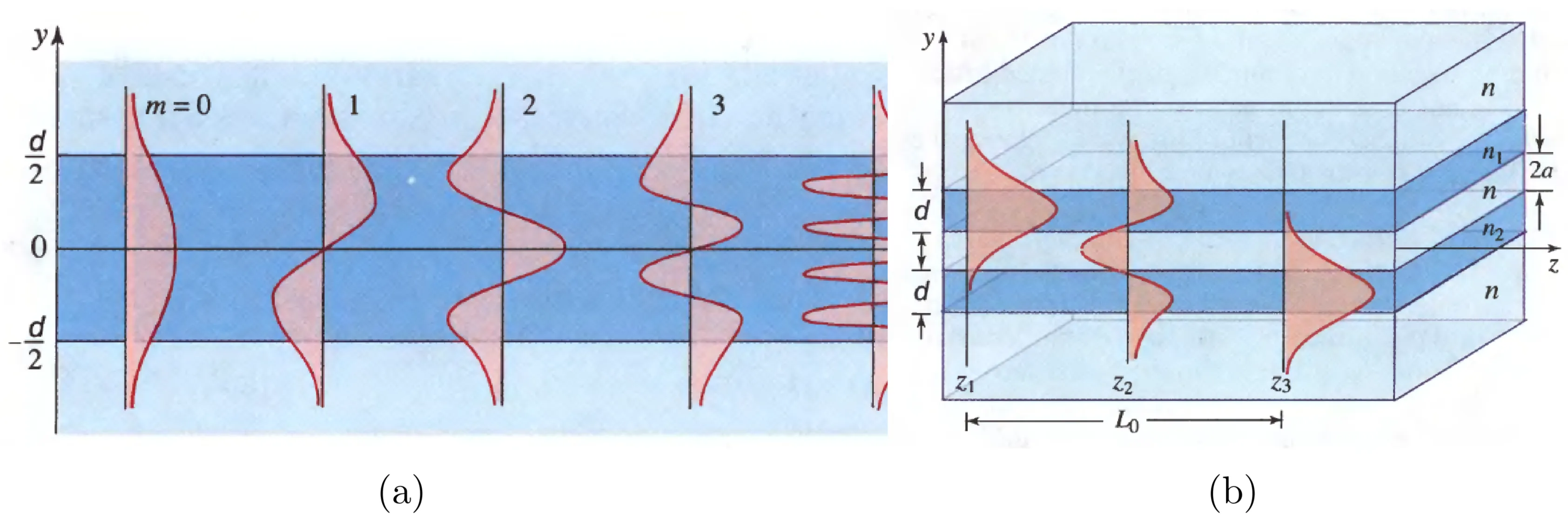
This is shown in the following figure (assuming
The associated magnetic field will have a non-zero
Planar mirror waveguides support a finite number of propagating modes
Thus, for a sufficiently thin waveguide (
10.1.2 TM Modes
For Transverse Magnetic (TM) modes, the magnetic field is transverse to
For
For
The exact coefficients and signs depend on normalisation and specific field component definitions. Thus, for each mode number
10.1.3 Dispersion Relation
The propagation constant
This is the dispersion relation for the
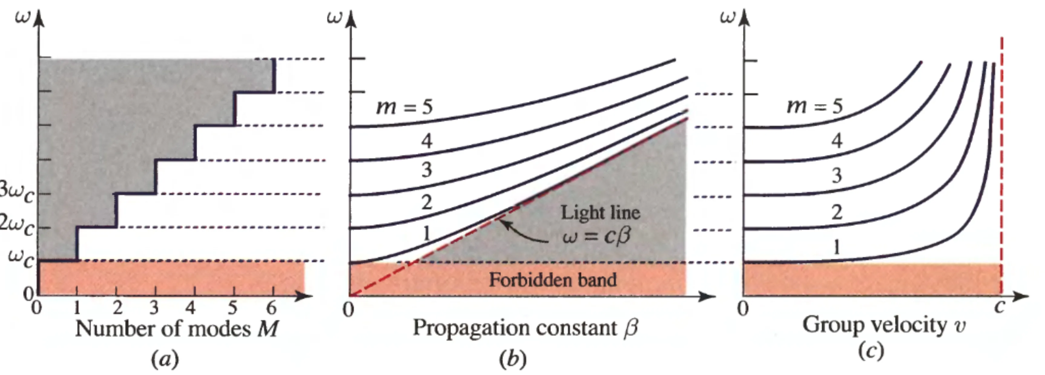
We observe in (b) that dispersion diagrams for different modes
An effective refractive index
where
10.1.4 Group and Phase Velocity
The group velocity
where
The phase velocity for mode
Since
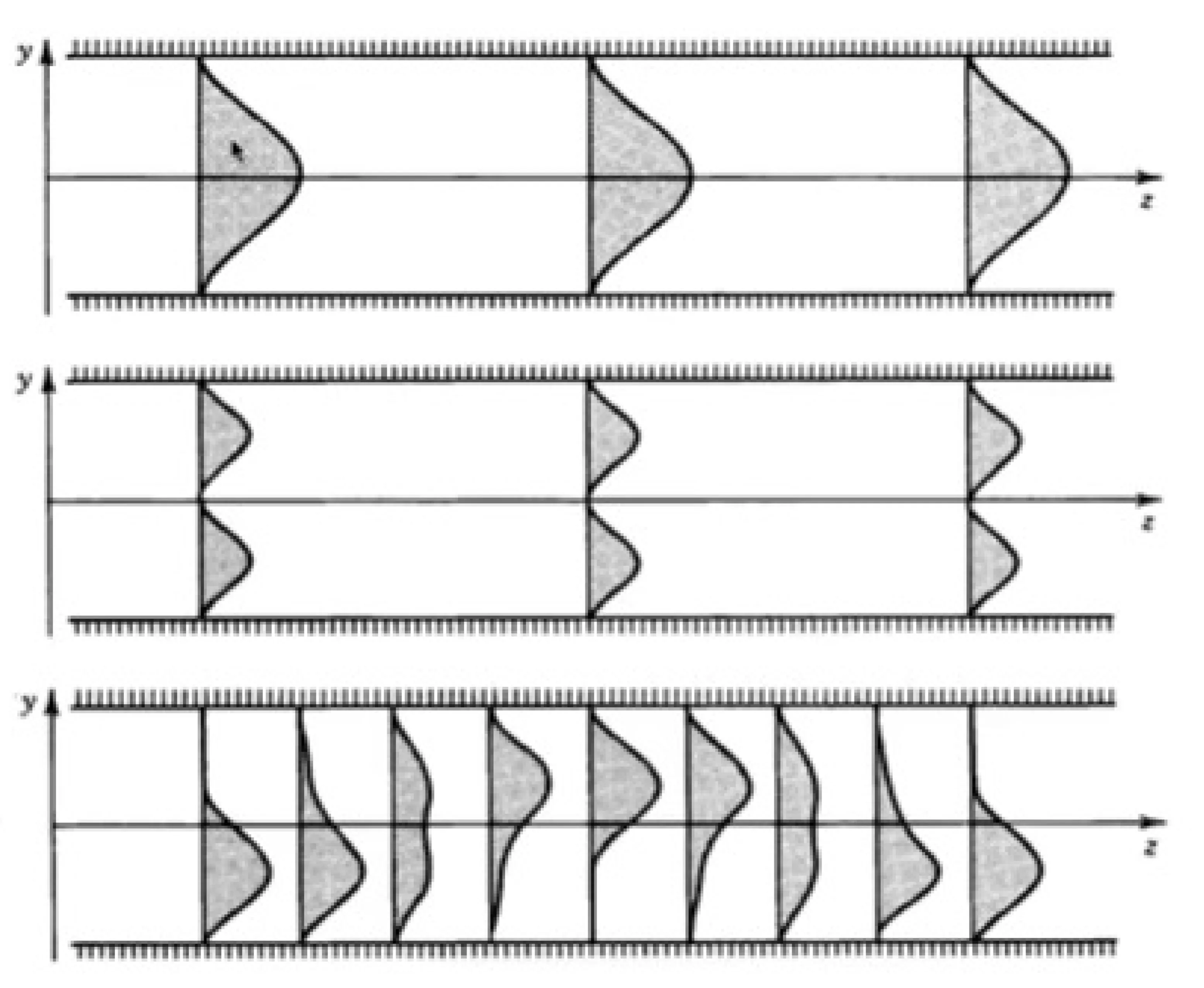
10.1.5 Multimode Fields
Generally, any field distribution that satisfies the boundary conditions (vanishes at the mirrors) will be guided. Such arbitrary fields can be expressed as a linear superposition of the allowed TE and TM modes. The transverse field profile of an arbitrary guided waveform will evolve with propagation distance
10.2 Planar Dielectric Waveguide
Planar waveguides are practically implemented using transparent dielectric materials with generally differing refractive indices. A common structure is a slab waveguide, consisting of a core layer with refractive index
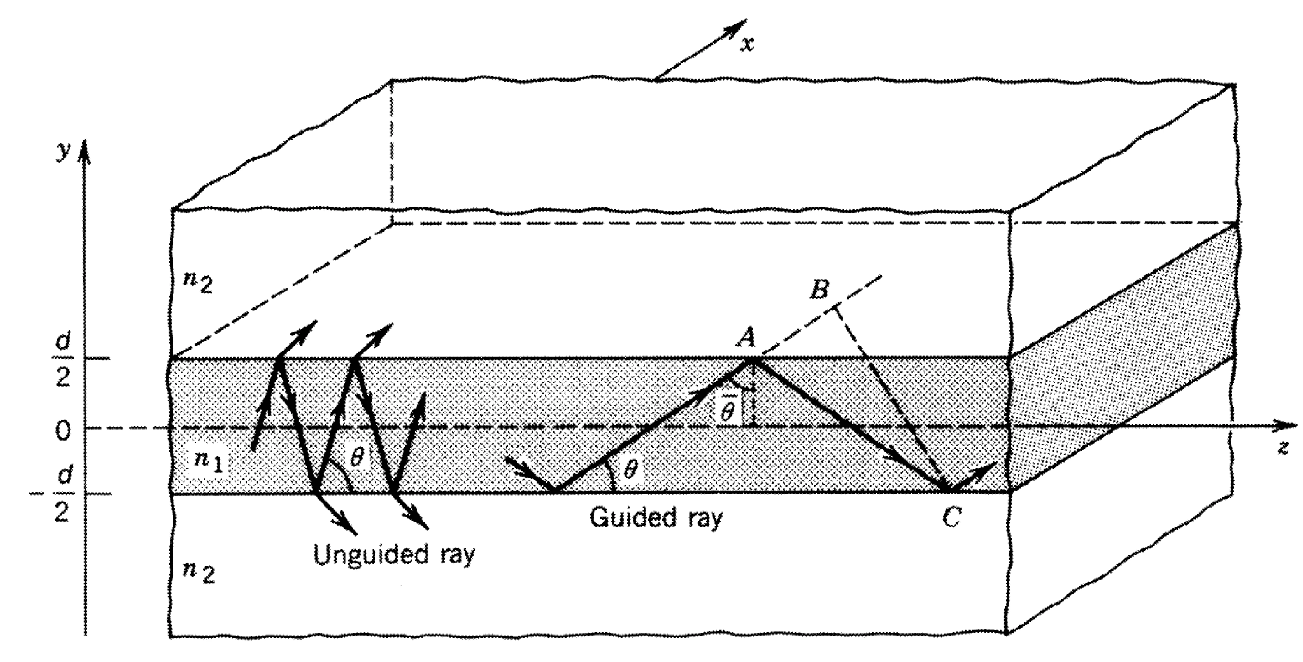
Light is guided within the core by total internal reflection (TIR) at the core-cladding interfaces. Rays incident on the interface from within the core at an angle
Similarly to the mirror waveguide, we seek self-consistent modes. However, an important difference is that upon total internal reflection, the reflected beam experiences a phase shift
A wave trapped within the waveguide core experiences this phase shift at each reflection. The condition for a guided mode is that the total phase change over a round trip in the transverse direction (including reflection phases) must be an integer multiple of
These equations are difficult to solve analytically and are typically solved graphically or numerically:
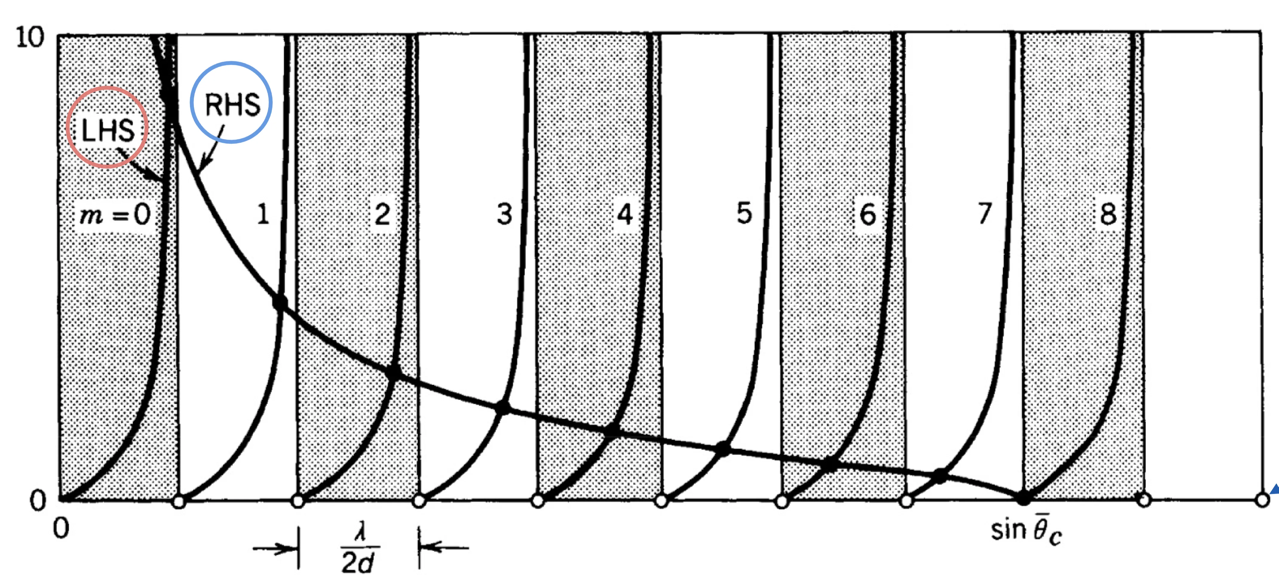
There is a finite number
This leads to a cutoff condition for each mode. The fundamental mode (m=0 for TE, in symmetric slab) has no cutoff frequency if
The dispersion diagram for a dielectric slab waveguide shows modes confined between the light line of the cladding (
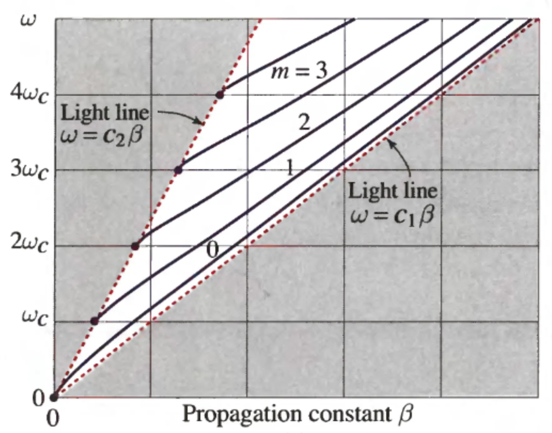
The effective refractive index
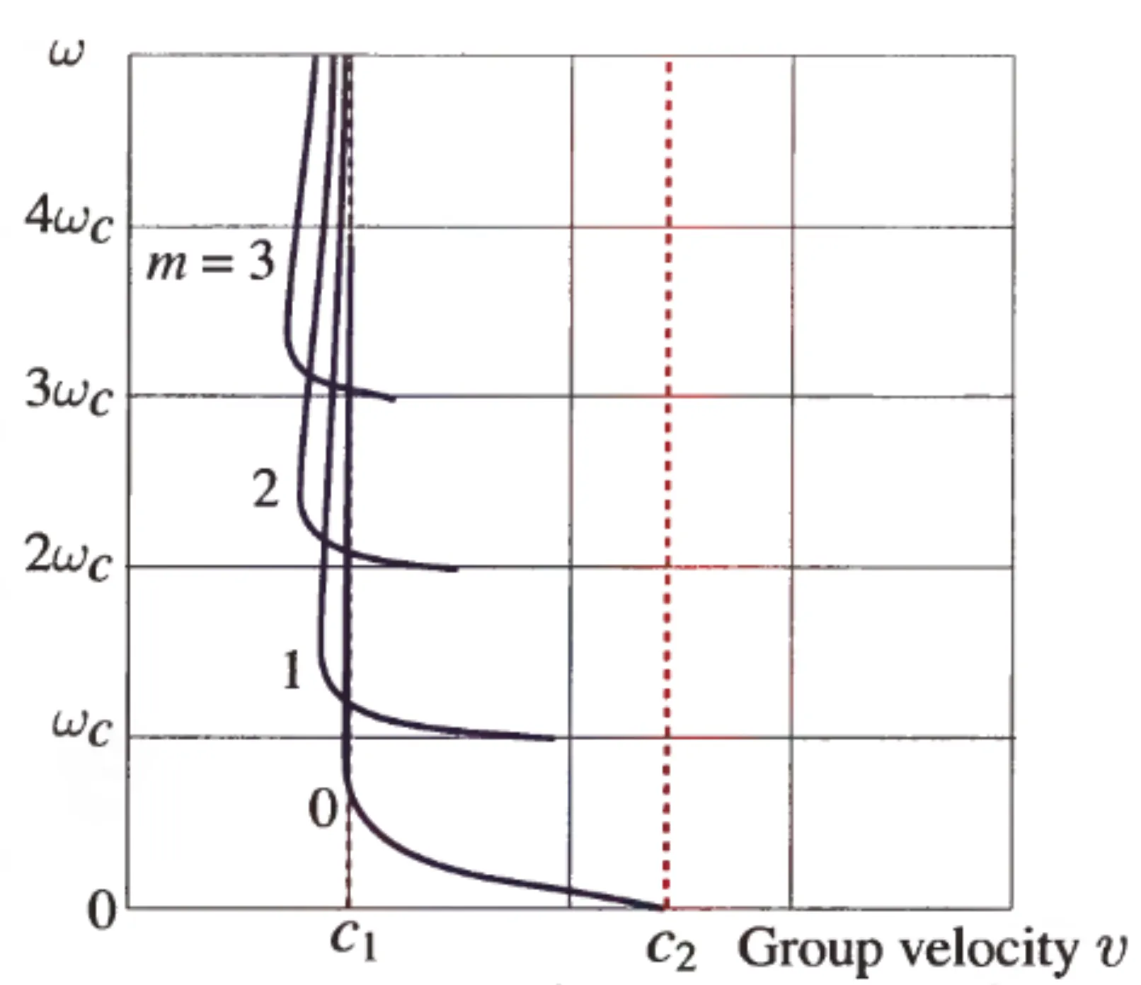
The group velocity
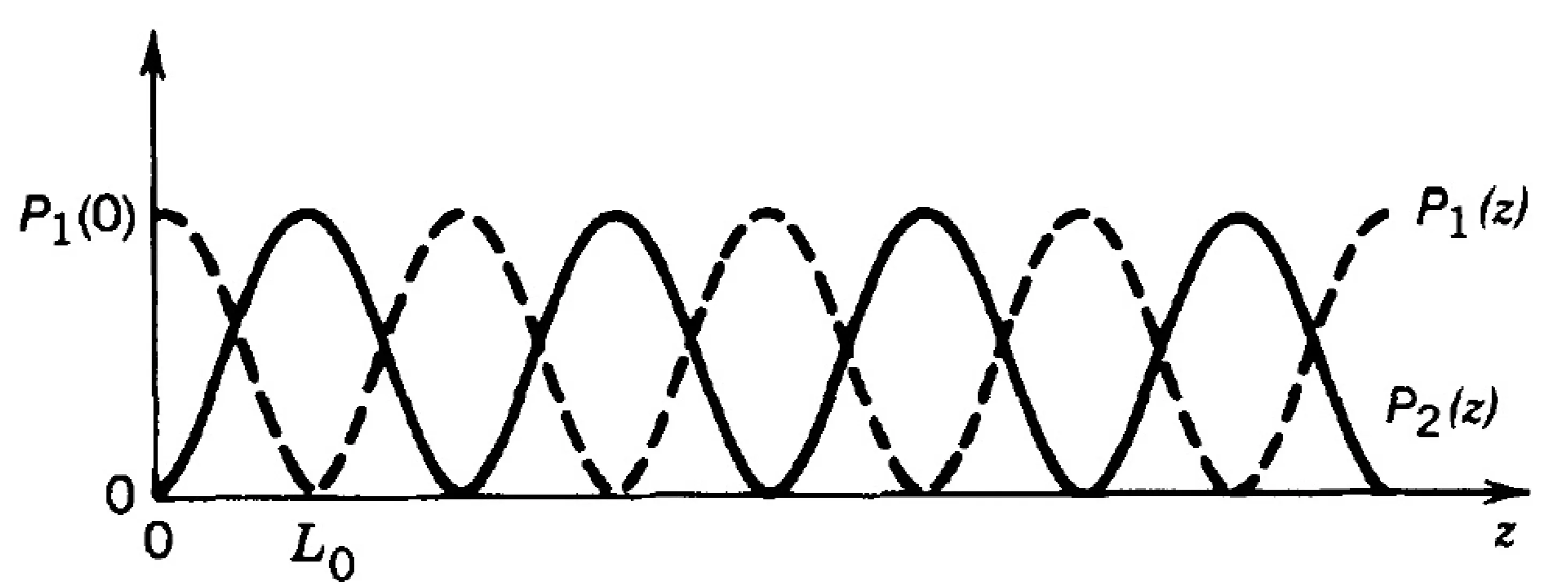
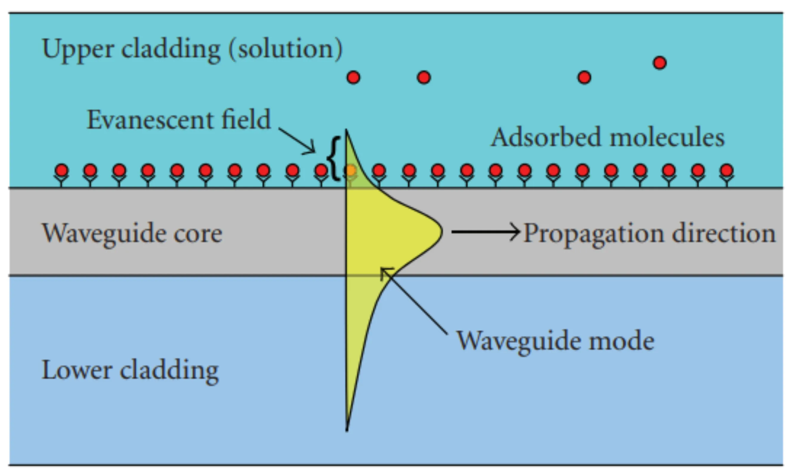
A key feature of dielectric waveguides is the presence of evanescent tails of the guided modes extending into the cladding region, even under TIR conditions. The field in the cladding decays exponentially with distance from the interface. This allows for evanescent field coupling if another waveguide is brought sufficiently close:
This coupling causes optical power to oscillate periodically between the two waveguides, forming the basis of directional couplers, which act as beamsplitters or power taps in integrated optics. Evanescently coupled waveguide arrays can also demonstrate coherence properties of light and are used in sensing applications, where changes in the cladding medium near the surface (such as binding of molecules) alter the effective index of the guided mode, leading to a measurable phase shift.

10.2.1 Numerical Aperture
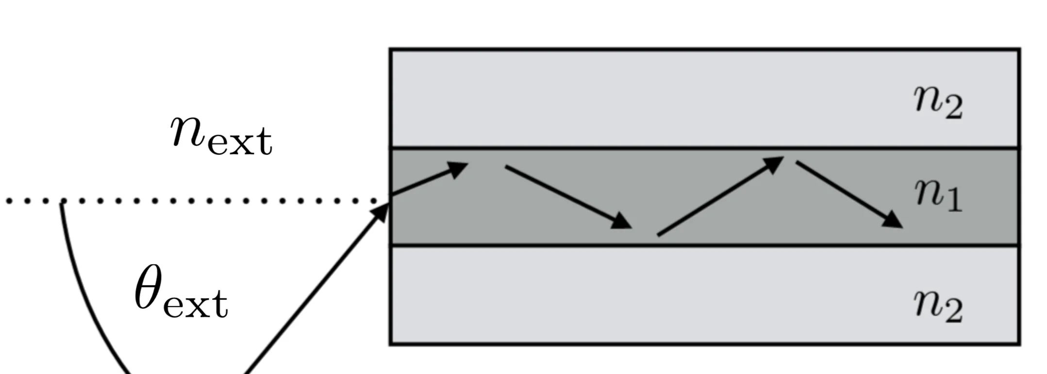
The numerical aperture (NA) is a measure of the light-gathering ability of an optical system, including waveguides. For a waveguide, it defines the maximum acceptance angle
For a planar dielectric slab waveguide with core index
This determines the cone of acceptance for efficient input coupling and also the divergence cone of light exiting the waveguide into free space.
10.2.2 Integrated Waveguides
A rapidly growing field in photonics is integrated optics, aiming to create compact optical circuits on a chip that guide, modulate, switch, and process light signals. These are often based on dielectric strip or channel waveguides.
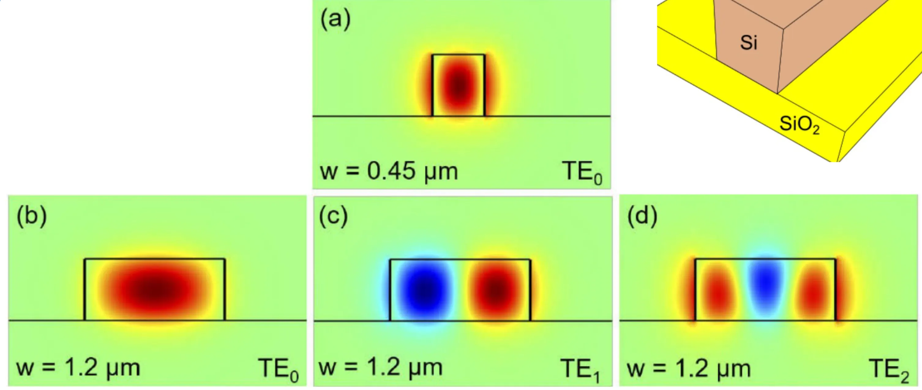
Higher refractive index contrast between the core and cladding allows for stronger mode confinement, enabling tighter bends and more compact device footprints. The image below shows different modes that can be confined in a strip waveguide made of Si on SiO
10.3 Optical Fibres
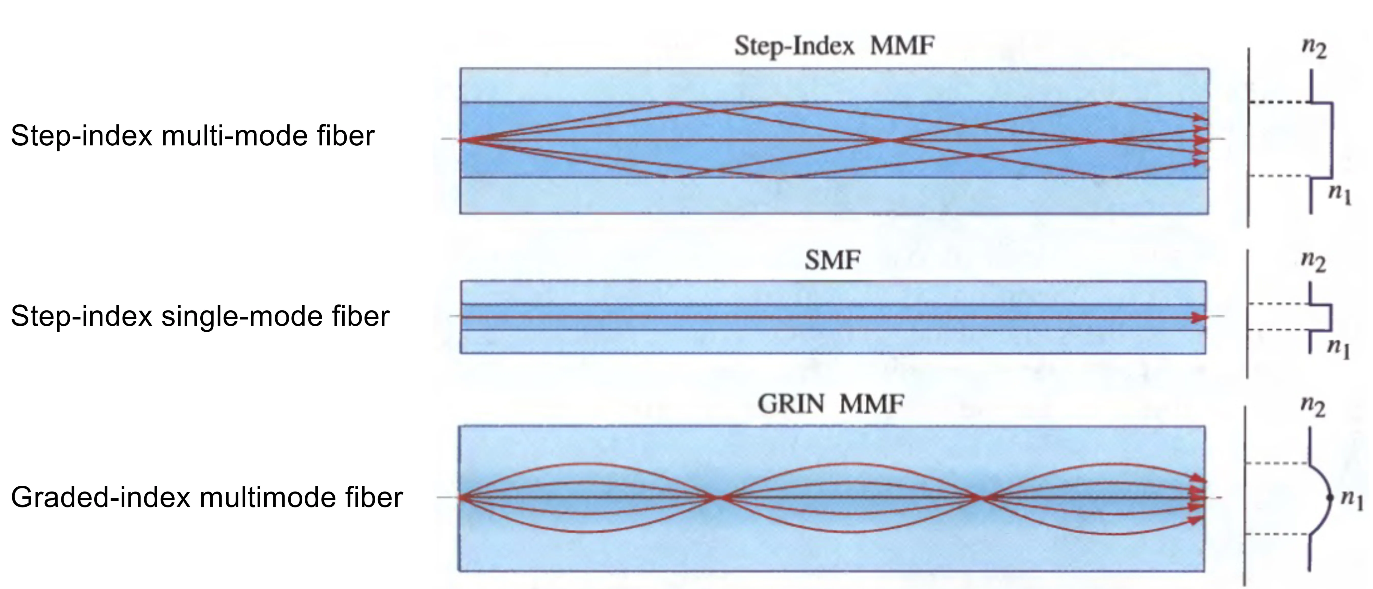
Optical fibres are a crucial class of cylindrical waveguides, essential for long-distance telecommunication and many other applications. Most common are step-index fibres, where a cylindrical core of higher refractive index
The refractive index difference
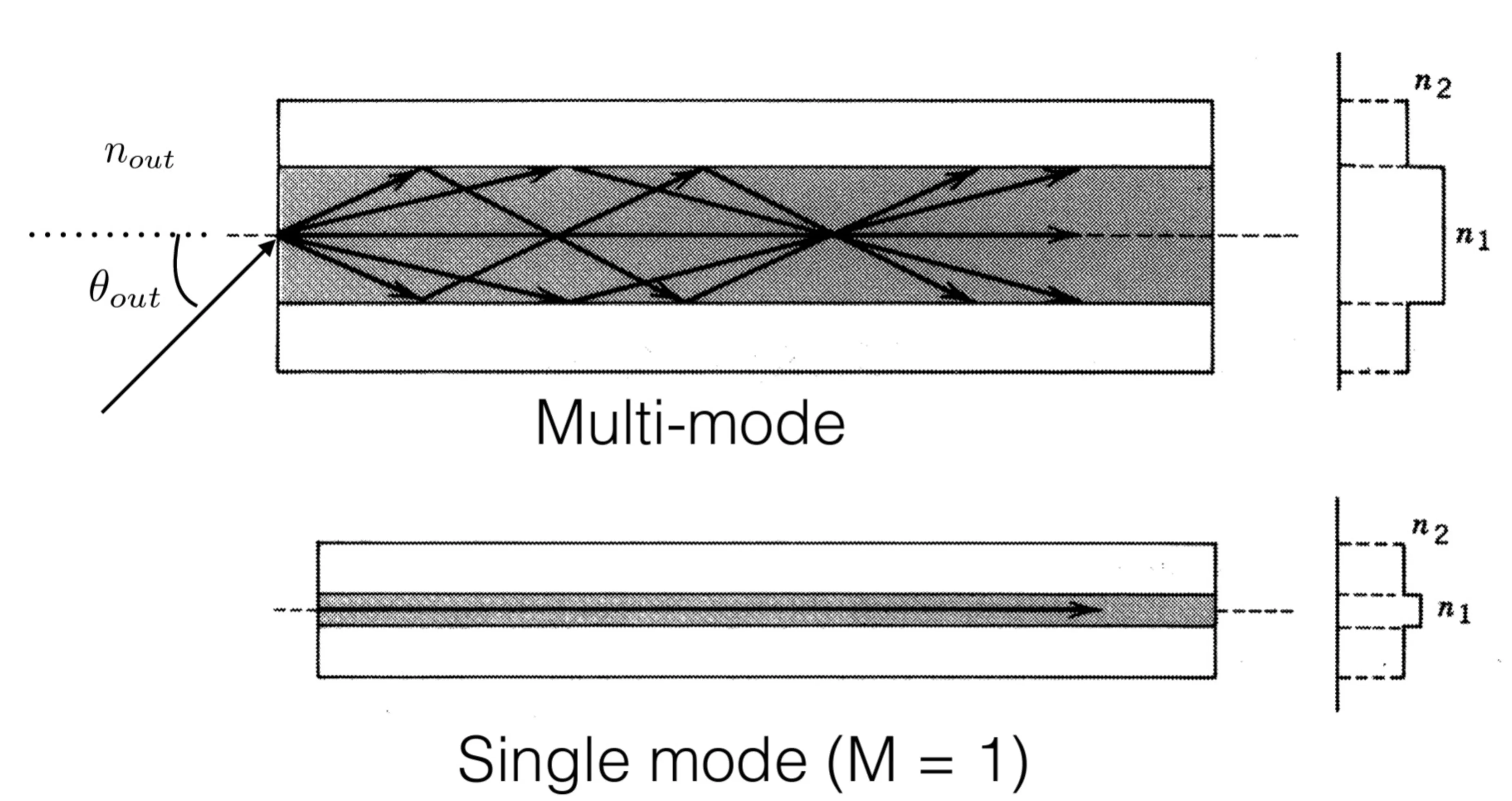
The guiding principle is total internal reflection at the core-cladding interface for rays incident at sufficiently grazing angles. The number of guided modes depends on the core diameter
- Single-mode fibres (SMFs) are designed with a small core diameter to support only the fundamental mode (typically
) for a given wavelength. - Multi-mode fibres (MMFs) have larger cores and support many modes.
The output of an SMF is approximately Gaussian in its transverse profile, which is beneficial for beam quality. MMFs suffer from modal dispersion (different modes travel at different group velocities), which limits their bandwidth for long-distance communication.
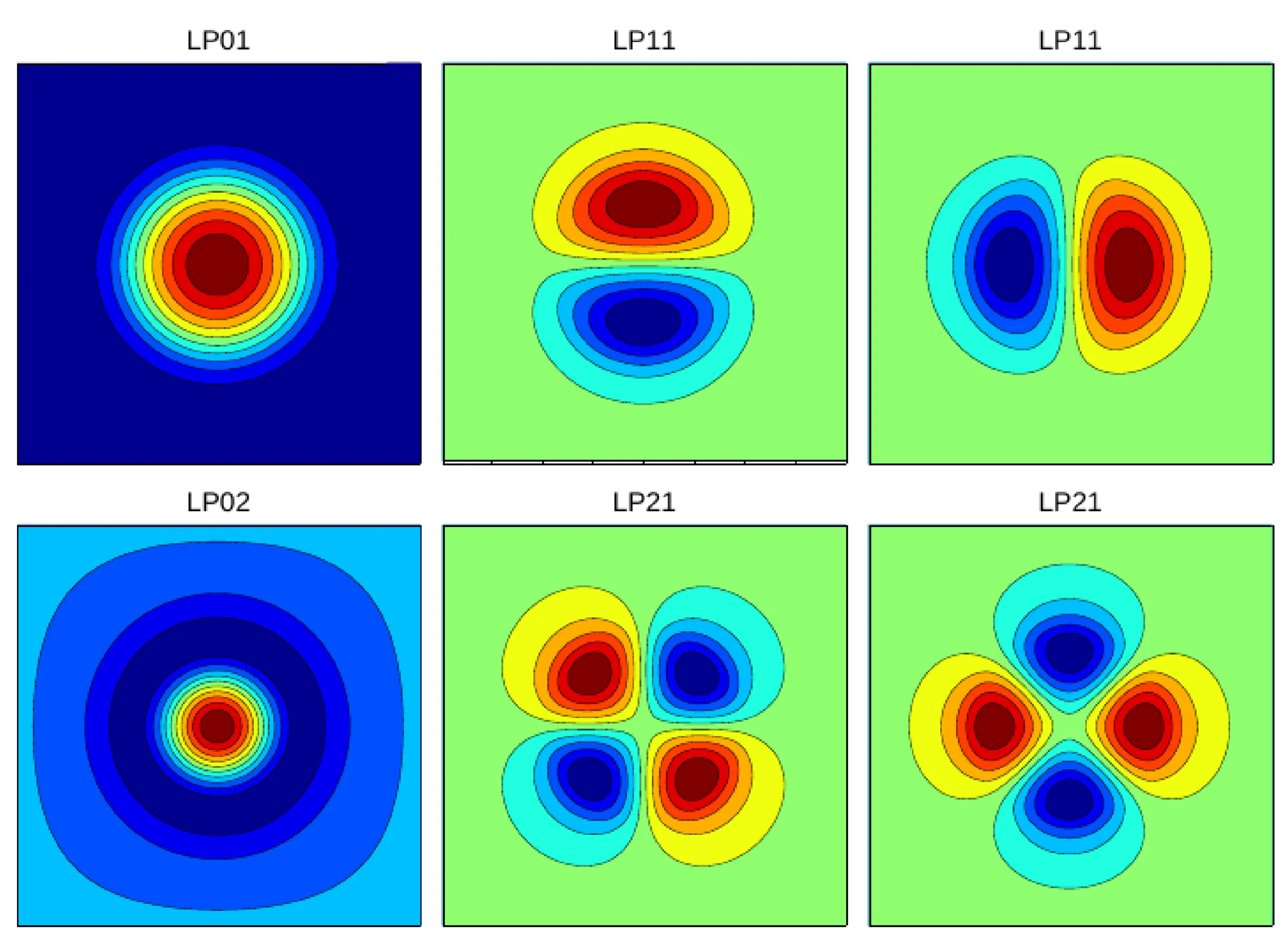
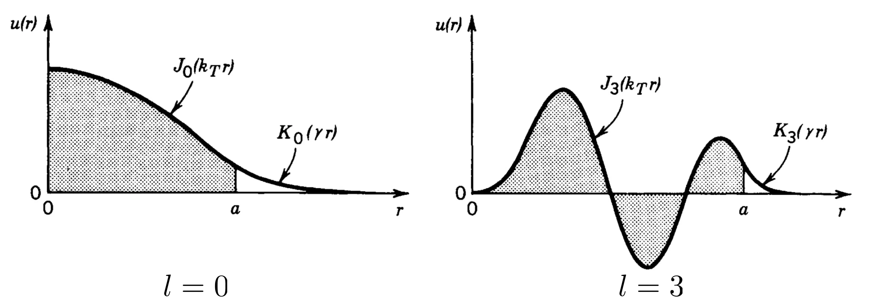
The field distributions for the lowest-order modes in a step-index optical fibre are described by Bessel functions in the core and modified Bessel functions in the cladding. Under the weak guiding approximation (
A fibre is single-mode if the normalised frequency or V-parameter satisfies:
where
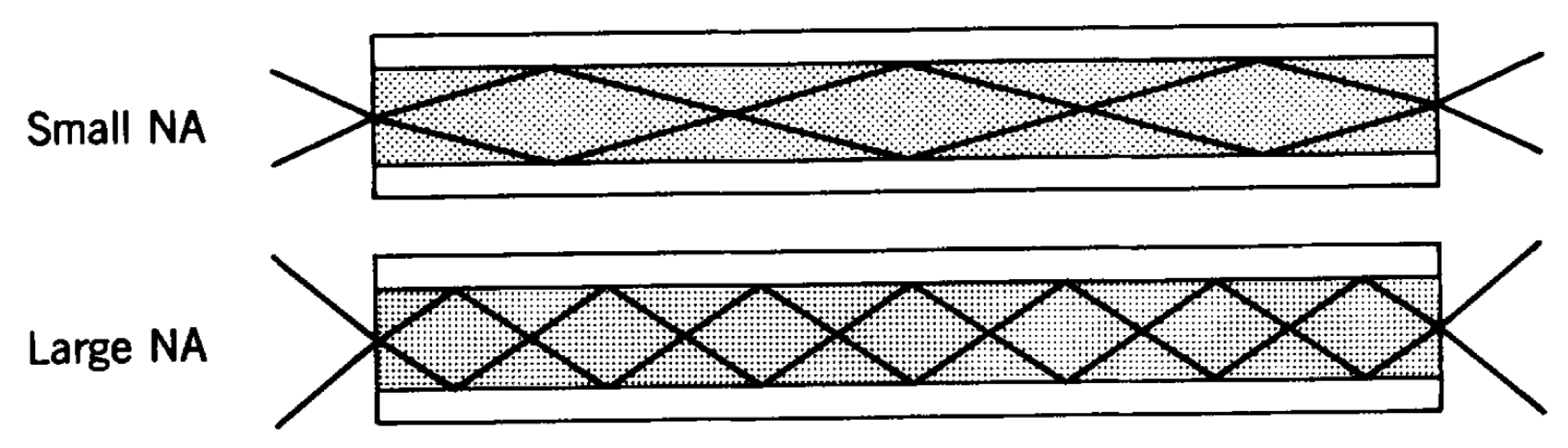
Analogous to the planar dielectric waveguide, light from outside is accepted into the fibre if its angle of incidence
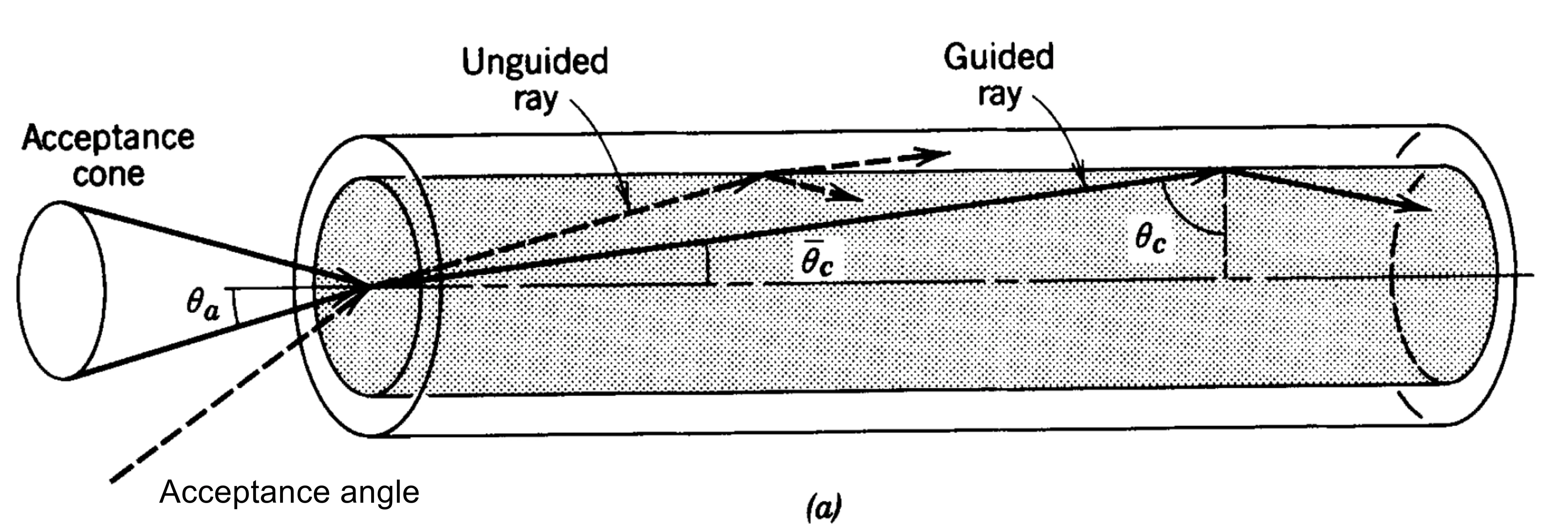
A large NA corresponds to a wider acceptance cone, making it easier to couple light into the fibre, but often implies higher potential for modal dispersion in MMFs or different guiding properties.
The radial part of the field solutions
where
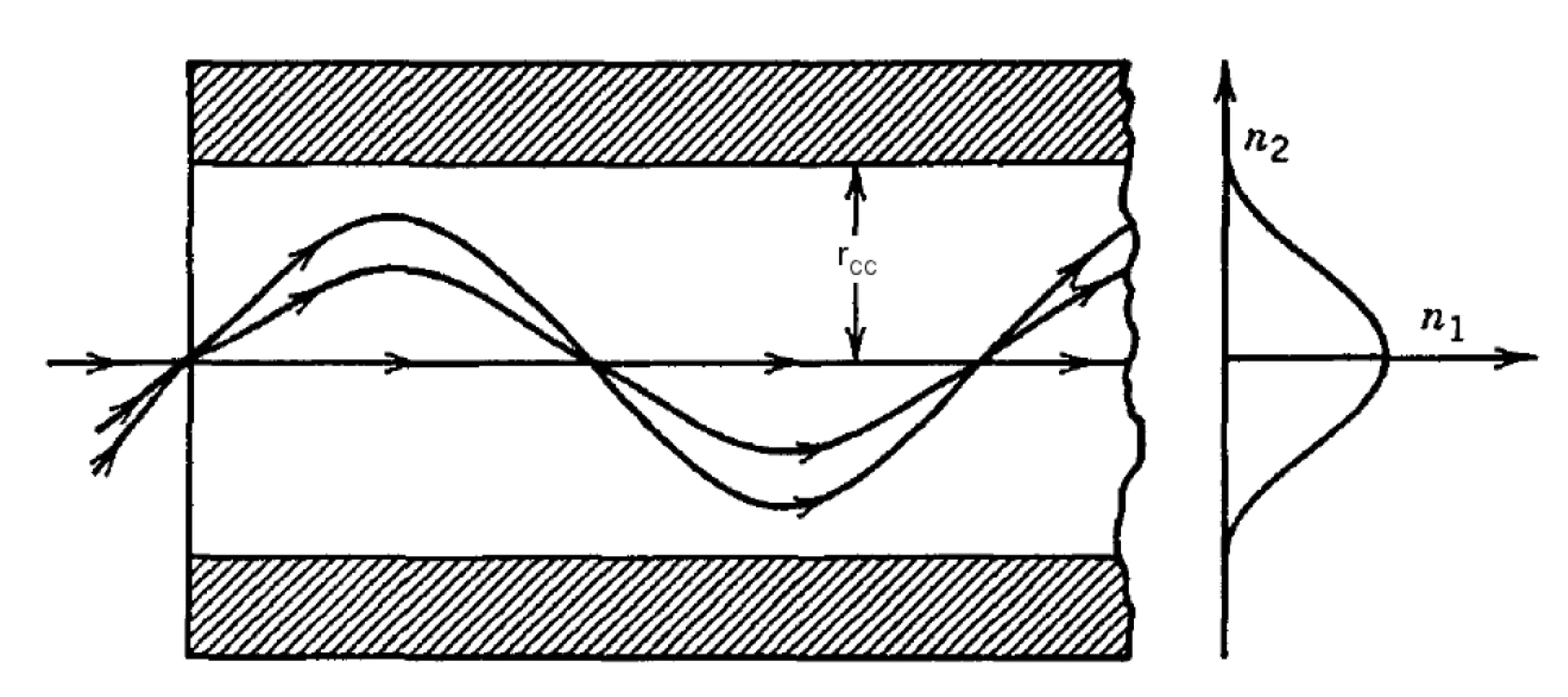
10.3.1 Graded-Index Fibres
Another type of optical fibre is the graded-index fibre (GRIN fibre), where the refractive index of the core
Typically, optical fibres also include an outer protective coating or 'jacket' for mechanical strength and protection.
10.3.2 Fibre Losses
For telecommunication applications transmitting signals over many thousands of kilometres, minimising fibre losses is crucial. Typically, a constant intrinsic loss coefficient
where
The attenuation coefficient
- Material absorption: Intrinsic absorption in the fibre material (such as silica), particularly from OH- ion impurities or UV/IR absorption tails.
- Rayleigh scattering: Scattering from microscopic density fluctuations frozen into the glass structure, scaling as
. This is dominant at shorter visible/near-IR wavelengths. - Waveguide imperfections / Mie scattering: Scattering from imperfections at the core-cladding interface or from larger-scale refractive index variations.
- Bending losses: Radiative losses incurred when the fibre is bent too tightly.
- Interface/Coupling losses: Losses at connections between fibres or to other optical elements.
Since losses often involve exponential power drop, decibel (dB) units are commonly used:
where
Logarithmic units simplify calculations for cascaded elements, turning multiplications into additions.
10.3.3 Polarisation-Maintaining Fibre
Standard single-mode fibres can exhibit random birefringence due to imperfections or stress, leading to a change in the polarisation state of light as it propagates. To maintain a specific input polarisation state throughout the fibre, Polarisation-Maintaining Fibres (PMFs) are used. These fibres have a controlled, strong internal birefringence intentionally introduced into their structure, for instance by using an elliptical core or by incorporating stress-applying elements alongside the core. This creates two well-defined principal polarisation axes (fast and slow). Light linearly polarised along one of these principal axes will largely maintain its polarisation state during propagation. Usually, the slow axis is used for launching light as it can be more robust against minor external perturbations.