Jump back to chapter selection.

Table of Contents

1.1 Microscopic Form of Maxwell's Equations in Vacuum
1.2 Maxwell's Equations in a Medium
1.3 The Material Equations
1.4 Macroscopic Approximation
1.5 Wave Equation
1.6 Solutions to the wave equation
1.7 Polarisation
1.8 Poynting Vector and Poynting's Theorem
1.9 Timescales
1.10 Momentum of Light

1 Electromagnetic Theory of Light

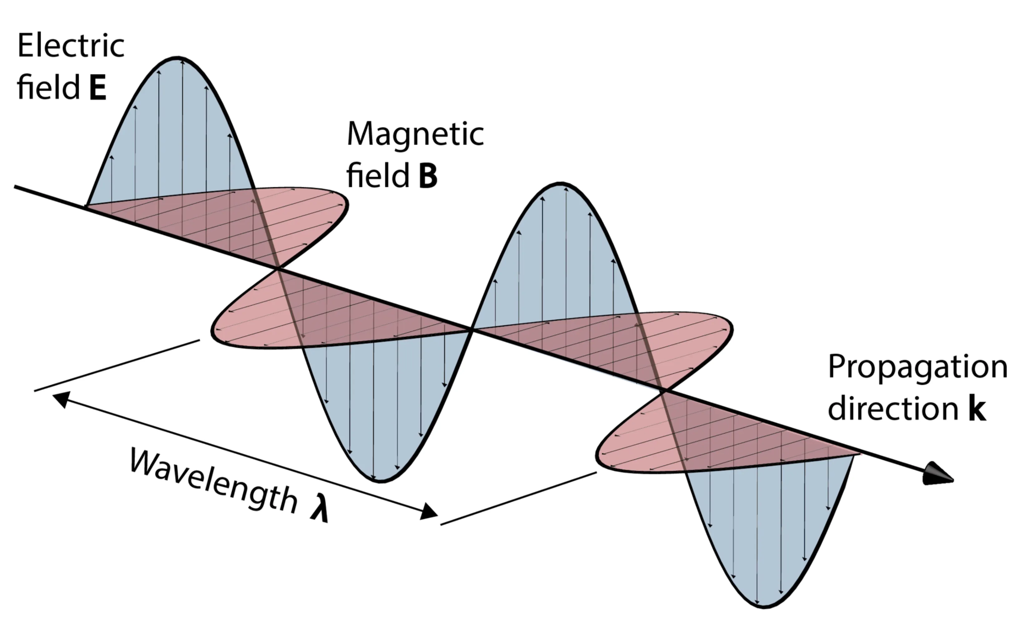
Light is an electromagnetic wave governed by the same theoretical principles that describe all forms of electromagnetic radiation. It consists of coupled oscillating electric and magnetic fields.

1.1 Microscopic Form of Maxwell's Equations in Vacuum

We begin with the simplest case by considering the electric and magnetic fields in free space, meaning there are no charges or currents present. The governing equations are Maxwell's equations:

Here, ${\epsilon }_0$ is the permittivity of free space, and ${\mu }_0$ is the permeability of free space. These equations describe how the electric field $\mathbf{E}$ and the magnetic field $\mathbf{B}$ evolve in time and space, with both fields being functions of position and time, so that $\mathbf{E}(\mathbf{r},t)$ and $\mathbf{B}(\mathbf{r},t)$.

A key property of Maxwell's equations is their linearity: any linear combination of solutions remains a valid solution. This has important implications, as we will see later. These equations have been experimentally confirmed for over a century and are fundamental to classical electrodynamics.

1.2 Maxwell's Equations in a Medium

To describe electromagnetic waves in a medium, we need a framework that accounts for the charge densities and currents at the atomic scale. The microscopic form of Maxwell's equations in a medium is given by:

where $\mathbf{j}$ is the total microscopic current density and $\rho$ is the total microscopic charge density. It is worth giving a meaning to each equation:

1. Gauss' Law: The electric field originates from charges. Positive charges act as sources, and negative charges act as sinks. The flux of $\mathbf{E}$ through a closed surface is proportional to the enclosed charge.
2. Gauss' Law for Magnetism: There are no magnetic monopoles; magnetic field lines always form closed loops. This distinguishes magnetic fields from electric fields, which can have isolated point sources (charges).
3. Faraday's Law of Induction: A time-dependent magnetic field creates a circulating electric field. This principle underlies electromagnetic induction, which is the basis of electrical generators, transformers, and inductors.
4. Ampère-Maxwell Law: Magnetic fields are produced both by electric currents and by changing electric fields. The latter term, ${\epsilon }_0\frac{\partial \mathbf{E}}{\partial t}$, is known as the displacement current density and allows electromagnetic waves to propagate even in the absence of actual charge flow.

While these equations describe the fundamental behaviour of electric and magnetic fields, solving them exactly in a material by tracking every individual charge is impractical. Instead, we often work with macroscopic versions of Maxwell’s equations. To achieve this, we introduce two auxiliary fields: the electric displacement field $\mathbf{D}$ and the magnetic field $\mathbf{H}$ (sometimes called magnetic field intensity). These quantities result from an effective spatial averaging of the microscopic fields over volumes that are large compared to atomic dimensions but small compared to the wavelength of the electromagnetic fields. This averaging is justified since atomic-scale structures are typically on the order of Angstroms or nanometres, whereas relevant optical wavelengths are often hundreds of nanometres or larger.

The macroscopic fields are defined as:

where $\mathbf{P}$ is the electric polarisation density (electric dipole moment per unit volume), and $\mathbf{M}$ is the magnetisation density (magnetic dipole moment per unit volume). These definitions allow us to describe the response of the medium without explicitly tracking all individual microscopic charges and currents. In a dielectric medium, the polarisation $\mathbf{P}$ is the macroscopic sum of the electric dipole moments induced by the electric field. The magnetisation $\mathbf{M}$ is defined analogously for magnetic materials. Both the displacement field $\mathbf{D}$ and the magnetic field $\mathbf{H}$ are often referred to as auxiliary fields. The polarisation and magnetisation are related to the electric field $\mathbf{E}$ and magnetic induction $\mathbf{B}$ through material-dependent relations called constitutive relations. In free space, both polarisation $\mathbf{P}$ and magnetisation $\mathbf{M}$ are zero, so $\mathbf{D}={\epsilon }_0\mathbf{E}$ and $\mathbf{H}=\mathbf{B}/{\mu }_0$.

In this course, we will be mainly concerned with isotropic media, meaning that the material response is independent of direction. This implies that the dielectric function ${\epsilon }_r(\mathbf{r},t)$ (relative permittivity) and the relative permeability ${\mu }_r(\mathbf{r},t)$ are scalars (or tensors that reduce to scalars). Furthermore, in many practical optical problems, it is sufficient to solve for the electric field alone. This is because in the non-relativistic regime, the force exerted by the magnetic component of light on charges is often much weaker than that of the electric component for many interactions. This assumption is further justified by the fact that most materials relevant to optics are non-magnetic at optical frequencies. However, one must always keep in mind the presence and role of the magnetic field.

1.3 The Material Equations

Solving Maxwell's equations in a medium requires explicit relationships, known as material or constitutive equations, which describe how the medium responds to the fields. As mentioned earlier, these relationships depend on the material properties. To establish the macroscopic Maxwell's equations, we begin by separating both the total charge density $\rho$ and the total current density $\mathbf{j}$ into free and bound contributions:

Free charges and currents are typically those that can move over macroscopic distances (like conduction electrons in a metal), while bound charges and currents are associated with localised atomic or molecular dipoles.

Our goal is to reformulate Maxwell's equations so that only free charges and currents appear explicitly as sources.
Starting from Gauss' Law in a medium, $\mathrm{\nabla }\cdot \mathbf{E}=({\rho }_f+{\rho }_b)/{\epsilon }_0$, we can write ${\epsilon }_0\mathrm{\nabla }\cdot \mathbf{E}-{\rho }_b={\rho }_f$.
By defining the polarisation density $\mathbf{P}$ such that the bound charge density is given by

we substitute this into Gauss' Law: ${\epsilon }_0\mathrm{\nabla }\cdot \mathbf{E}+\mathrm{\nabla }\cdot \mathbf{P}={\rho }_f$. This can be rewritten using the electric displacement $\mathbf{D}={\epsilon }_0\mathbf{E}+\mathbf{P}$ as

At this point, we have successfully removed explicit dependence on the bound charges.
A similar approach applies to the Ampère-Maxwell Law. The total current $\mathbf{j}$ includes ${\mathbf{j}}_f$ and ${\mathbf{j}}_b$. The bound current density ${\mathbf{j}}_b$ can be expressed in terms of polarisation $\mathbf{P}$ and magnetisation $\mathbf{M}$ as

Substituting this into the microscopic Ampère-Maxwell Law $\mathrm{\nabla }\times \mathbf{B}={\mu }_0({\mathbf{j}}_f+{\mathbf{j}}_b+{\epsilon }_0\frac{\partial \mathbf{E}}{\partial t})$:

Rearranging gives $\mathrm{\nabla }\times (\frac{\mathbf{B}}{{\mu }_0}-\mathbf{M})={\mathbf{j}}_f+\frac{\partial ({\epsilon }_0\mathbf{E}+\mathbf{P})}{\partial t}$.
Using the definitions of $\mathbf{H}=\frac{1}{{\mu }_0}\mathbf{B}-\mathbf{M}$ and $\mathbf{D}={\epsilon }_0\mathbf{E}+\mathbf{P}$, this becomes

We can summarise the microscopic Maxwell's equations (which are universally valid) and the macroscopic Maxwell's equations (useful for describing fields in media):

Additionally, the auxiliary relations defining $\mathbf{D}$ and $\mathbf{H}$ are:

And the definitions relating bound sources to $\mathbf{P}$ and $\mathbf{M}$ are:

1.4 Macroscopic Approximation

The macroscopic quantities $\mathbf{P}$ and $\mathbf{M}$ (and thus $\mathbf{D}$ and $\mathbf{H}$) are obtained by averaging microscopic properties over physically infinitesimal volumes that are nevertheless large enough to contain many atoms or molecules. The total charge in a macroscopic volume $V$ at position $\mathbf{R}$ is

while the total current through a surface element associated with this volume is related to

The electric dipole moment of the volume $V$ is defined as

while the magnetic dipole moment is

The free charge and free current densities are then given by averages:

while the macroscopic polarisation and magnetisation are dipole moments per unit volume:

The macroscopic Maxwell equations effectively describe the fields averaged over these volumes. This approximation is valid as long as the fields do not vary significantly over the scale of the averaging volume.

To proceed further with solving problems, we require constitutive relations that link $\mathbf{P}$ to $\mathbf{E}$ and $\mathbf{M}$ to $\mathbf{H}$ (or $\mathbf{B}$). These relations depend on the material's properties and are often established through a set of approximations:

1. Electric and magnetic field dependence: It is often assumed that $\mathbf{P}$ depends primarily on $\mathbf{E}$ and not on $\mathbf{B}$, while $\mathbf{M}$ depends primarily on $\mathbf{B}$ (or $\mathbf{H}$) and not on $\mathbf{E}$. This is a good approximation for many materials at optical frequencies, although magneto-optic effects do exist where fields cross-couple.
2. Locality: $\mathbf{P}(\mathbf{r})$ and $\mathbf{M}(\mathbf{r})$ are assumed to depend only on the fields $\mathbf{E}(\mathbf{r})$ and $\mathbf{B}(\mathbf{r})$ at the same position $\mathbf{r}$. This implies that the response is local and bound charges/currents do not move significantly relative to the scale over which the fields change. This is part of the long-wavelength approximation (wavelength much larger than atomic scales). Spatial dispersion occurs when this is not true.
3. Homogeneity: The functional dependence of $\mathbf{P}$ and $\mathbf{M}$ on $\mathbf{E}$ and $\mathbf{B}$ respectively, does not vary with position $\mathbf{r}$ in the medium, implying the medium is optically homogeneous.
4. Instantaneous Response (No Temporal Dispersion): $\mathbf{P}$ and $\mathbf{M}$ at time $t$ are assumed to depend only on the values of $\mathbf{E}$ and $\mathbf{B}$ at the same time $t$, eliminating time integrals (convolutions) in the time domain. This assumption is only valid for optically transparent materials far from any absorption resonances. In reality, this is often a poor approximation for many materials over a broad range of frequencies, and temporal dispersion (frequency dependence of material parameters like ${\epsilon }_r(\omega )$) is crucial. This will be refined later.
5. Linearity: $\mathbf{P}$ and $\mathbf{M}$ are assumed to be linear functions of $\mathbf{E}$ and $\mathbf{B}$ (or $\mathbf{H}$), respectively. This is the domain of linear optics. Non-linear optics deals with higher-order dependencies.
6. Isotropy: The response of the medium is assumed to be independent of the direction of the applied fields. For isotropic media, $\mathbf{P}$ is parallel to $\mathbf{E}$, and $\mathbf{M}$ is parallel to $\mathbf{H}$ (or $\mathbf{B}$). This means susceptibilities and permittivities can be treated as scalars. This assumption is violated in anisotropic materials like many crystals.

Let us examine the effect of these assumptions. With assumption 1, we may generally write the response as a functional of the field history. For instance:

With assumptions 2, 3, and 4 (locality, homogeneity, and instantaneous response), these simplify to:

With assumption 5 (linearity), we can expand $\mathbf{P}$ and $\mathbf{M}$ in a Taylor series and keep only the linear terms (assuming no permanent dipole moments $P^{(0)},M^{(0)}$, or that they are zero for symmetry reasons):

Here, ${\chi }_{ij}^{(1)}$ is the linear electric susceptibility tensor and ${\chi }_{ij}^{(m1)}$ is the linear magnetic susceptibility tensor. Higher-order terms (like ${\chi }^{(2)},{\chi }^{(3)}$) are the focus of non-linear optics, but for this course, low-intensity light and linear responses are generally assumed unless stated otherwise.
Finally, with assumption 6 (isotropy), the susceptibility tensors reduce to scalars multiplied by the identity tensor, so ${\chi }_{ij}^{(1)}=\chi {\delta }_{ij}$ and ${\chi }_{ij}^{(m1)}={\chi }_m{\delta }_{ij}$. This leads to:

The relative permittivity (dielectric constant) ${\epsilon }_r$ and relative permeability ${\mu }_r$ are then defined as:

Therefore, we can write the macroscopic constitutive relations as:

In optics, we generally deal with non-magnetic media, so $\mathbf{M}\approx 0$, which implies ${\chi }_m\approx 0$ and thus ${\mu }_r\approx 1$. In such cases, $\mathbf{B}\approx {\mu }_0\mathbf{H}$.

1.5 Wave Equation

To describe the propagation of light, we seek an equation that relates the temporal evolution of the fields to their spatial variation. We derive this for the case of a homogeneous, isotropic, linear, and non-magnetic (${\mu }_r=1$) medium, with no free charges (${\rho }_f=0$) or free currents (${\mathbf{j}}_f=0$), and initially assuming no dispersion (so ${\epsilon }_r$ is constant).
Consider the macroscopic curl equation (Faraday's Law):

Apply the curl operator to both sides:

Using the vector identity $\mathrm{\nabla }\times (\mathrm{\nabla }\times \mathbf{A})=\mathrm{\nabla }(\mathrm{\nabla }\cdot \mathbf{A})-{\mathrm{\nabla }}^2\mathbf{A}$, the left side becomes $\mathrm{\nabla }(\mathrm{\nabla }\cdot \mathbf{E})-{\mathrm{\nabla }}^2\mathbf{E}$.
Since ${\rho }_f=0$ and the medium is homogeneous, $\mathrm{\nabla }\cdot \mathbf{D}={\epsilon }_0{\epsilon }_r\mathrm{\nabla }\cdot \mathbf{E}=0$, which implies $\mathrm{\nabla }\cdot \mathbf{E}=0$.
Thus, $\mathrm{\nabla }\times (\mathrm{\nabla }\times \mathbf{E})=-{\mathrm{\nabla }}^2\mathbf{E}$.
For the right side, we use the Ampère-Maxwell Law (macroscopic, no free currents): $\mathrm{\nabla }\times \mathbf{H}=\frac{\partial \mathbf{D}}{\partial t}$.
Since $\mathbf{B}={\mu }_0\mathbf{H}$ (for ${\mu }_r=1$) and $\mathbf{D}={\epsilon }_0{\epsilon }_r\mathbf{E}$, we have $\mathrm{\nabla }\times \mathbf{B}={\mu }_0\frac{\partial ({\epsilon }_0{\epsilon }_r\mathbf{E})}{\partial t}={\mu }_0{\epsilon }_0{\epsilon }_r\frac{\partial \mathbf{E}}{\partial t}$.
Substituting these into the curled Faraday's Law:

This yields the wave equation for $\mathbf{E}$:

A similar derivation yields the wave equation for $\mathbf{H}$ (or $\mathbf{B}$).
Both equations have the form of a generic linear wave equation. The wave propagation speed, or phase velocity $v_p$, in the medium is given by $v_p^2=1/({\mu }_0{\epsilon }_0{\epsilon }_r)$.
The speed of light $c$ in vacuum is given by $c^2=1/({\epsilon }_0{\mu }_0)$, so $c=1/\sqrt{{\epsilon }_0{\mu }_0}$.
The refractive index $n$ of the medium is defined as the ratio of the speed of light in vacuum to the phase velocity in the medium:

This uses the assumption of a non-magnetic medium (${\mu }_r=1$). Therefore, the wave equation can be written as:

1.6 Solutions to the wave equation

One fundamental solution of the wave equation is the monochromatic plane wave:

where ${\mathbf{E}}_0$ is the constant amplitude vector, $\omega$ is the angular frequency, $\mathbf{k}$ is the wavevector, and $\varphi$ is a phase constant. The angular frequency and the magnitude of the wavevector, $k=|\mathbf{k}|$, are related by the dispersion relation:

The relation between the wavenumber $k$ and the wavelength in the medium ${\lambda }_n$ is $k=2\pi /{\lambda }_n$. The wavelength in vacuum is ${\lambda }_0=n{\lambda }_n$.

The wave equation is linear (since derivatives are linear operators), and thus any superposition of solutions is also a solution. While plane waves are simple solutions, they form a complete basis, meaning any solution to the wave equation can be expressed as a linear combination (or integral) of plane waves (Fourier decomposition).
From $\mathrm{\nabla }\cdot \mathbf{E}=0$ (for a uniform medium with no free charges), it follows that plane waves are transverse:

For this to be zero at all times and positions, we require ${\mathbf{E}}_0\cdot \mathbf{k}=0$, meaning the electric field vector is perpendicular to the direction of propagation.
Similarly for the magnetic field, a solution is:

The electric and magnetic fields of a plane wave are not independent. From Maxwell's equation $\mathrm{\nabla }\times \mathbf{E}=-\frac{\partial \mathbf{B}}{\partial t}$, by substituting the plane wave solutions, we find the relation:

This implies that ${\mathbf{B}}_0$ is perpendicular to both $\mathbf{k}$ and ${\mathbf{E}}_0$. Therefore, for a plane wave in an isotropic medium, $\mathbf{E}$, $\mathbf{B}$, and $\mathbf{k}$ form a mutually orthogonal triad. This is illustrated in the next figure:

The relationship between the amplitudes can also be expressed using the wave impedance of the medium, $Z=\sqrt{\mu /\epsilon }=\sqrt{{\mu }_0{\mu }_r/{\epsilon }_0{\epsilon }_r}$. For non-magnetic media (${\mu }_r=1$), $Z=\sqrt{{\mu }_0/({\epsilon }_0{\epsilon }_r)}=Z_0/n$, where $Z_0=\sqrt{{\mu }_0/{\epsilon }_0}\approx 377\mathrm{\Omega }$ is the impedance of free space. Then $|{\mathbf{E}}_0|=Z|{\mathbf{H}}_0|$, and ${\mathbf{H}}_0=\frac{1}{Z}(\hat{\mathbf{k}}\times {\mathbf{E}}_0)$, where $\hat{\mathbf{k}}=\mathbf{k}/k$.
Because the electric and magnetic fields are orthogonal to the direction of propagation, these waves are also called transverse electro-magnetic (TEM) waves.
It is often more convenient to use complex notation:

where $\tilde{\mathbf{E}}(\mathbf{r})={\tilde{\mathbf{E}}}_0{e}^{i\mathbf{k}\cdot \mathbf{r}}$ is the complex amplitude (phasor), and ${\tilde{\mathbf{E}}}_0$ may itself be complex to include the phase constant $\varphi$. The physical field is obtained by taking the real part. Often, the $\mathfrak{Re}[\cdot ]$ is dropped for brevity in intermediate calculations, but it must be reinstated when calculating real physical quantities, especially those that depend nonlinearly on the fields, such as intensity or the Poynting vector.

1.7 Polarisation

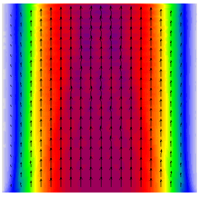
The polarisation of light describes the orientation of the electric field vector oscillation. For a plane wave propagating in the $z$-direction ($\mathbf{k}=k\hat{\mathbf{z}}$), the electric field vector ${\mathbf{E}}_0$ lies in the $x-y$ plane.
Linear polarisation means that the electric field vector oscillates along a fixed straight line in the $x-y$ plane:

where ${\alpha }_p$ is the angle of the polarisation direction with respect to the $x$-axis.

The underlying physics of how materials respond to polarised light relates to how their constituent charges (and thus dipole moments) interact with the electric field. A microscopic electric dipole moment is $\mathbf{p}=q\mathbf{L}$, where $q$ is charge and $\mathbf{L}$ is the vector separating charges. The macroscopic polarisation $\mathbf{P}$ is the vector sum of these microscopic dipole moments per unit volume: if there are $N$ dipoles per unit volume, and $⟨\mathbf{p}⟩$ is the average dipole moment, then $\mathbf{P}=N⟨\mathbf{p}⟩$.

Polarisation is important in the interaction of light with matter: the amount of light reflected from or transmitted through a surface depends on it (Fresnel equations), as does the amount of light absorbed in many materials. This is even more general - light scattering is often polarisation dependent. The refractive index itself can be polarisation dependent in anisotropic materials.
Light does not have to be linearly polarised. The general case is elliptical polarisation, where the tip of the electric field vector traces an ellipse in the $x-y$ plane over one optical cycle.

This can be best shown graphically. In the following figures (source), a wave oscillates (red) into the $z$-direction. The projections onto the $x$- and $y$-axis are in green and blue, respectively.

Linear polarisation - the total electric field vector oscillates along a straight line in the $x-y$ plane:

Elliptical polarisation - the total electric field vector traces an ellipse in the $x-y$ plane:

Circular polarisation - the total electric field vector traces a circle in the $x-y$ plane:

It becomes clear that circular polarisation is a special case of elliptical polarisation, where the $x$- and $y$-amplitudes of the electric field components are equal ($|E_{0x}|=|E_{0y}|$), and their phase difference is $\pm \pi /2$. The case of a $+\pi /2$ phase difference (e.g., $E_y$ leads $E_x$) can define right-hand circular polarisation (RHCP) by one convention, while a $-\pi /2$ phase difference defines left-hand circular polarisation (LHCP) (conventions vary, often depending on whether viewed from source or receiver).
A linear polariser is an optical element that transmits light of a specific polarisation while blocking light of the orthogonal polarisation. If $\hat{\mathbf{e}}$ is the unit vector along the transmission axis of the polariser, then for a given input electric field ${\mathbf{E}}_{\text{in}}$, the output field is its projection onto this axis:

If $\hat{\mathbf{e}}=\cos {\theta }_p\cdot \hat{\mathbf{x}}+\sin {\theta }_p\cdot \hat{\mathbf{y}}$, where ${\theta }_p$ is the angle of the polariser's axis with respect to the $x$-axis.

1.8 Poynting Vector and Poynting's Theorem

Light carries energy. The quantity quantifying the rate and direction of electromagnetic energy flow per unit area is the Poynting vector $\mathbf{S}$, defined for instantaneous real fields as:

Its units are Watts per square metre (W/m${}^2$). Note that for calculating instantaneous power flow, real physical fields $\mathbf{E}(\mathbf{r},t)$ and $\mathbf{H}(\mathbf{r},t)$ must be used, not their complex representations directly, as energy and power are real, non-linear quantities in terms of fields. The Poynting vector indicates that the energy flow is orthogonal to both the electric and magnetic fields.

The Poynting theorem expresses energy conservation for electromagnetic fields. It states that the rate of decrease of electromagnetic energy stored within a volume, plus the rate of energy flowing out through the surface of that volume, equals the rate of work done by the fields on the free charges within the volume:

The electromagnetic energy density $u$ in a linear, isotropic medium is given by:

The Poynting theorem represents the conservation or balance of energy: the power flow out of a volume plus the rate of increase of stored energy within that volume equals the negative of the power delivered to free charges (Ohmic losses if ${\mathbf{j}}_{\mathbf{f}}=\sigma \mathbf{E}$). This form is valid for media where $u$ is well-defined as above (e.g., non-dispersive or carefully treated dispersive cases). The term $-{\mathbf{j}}_{\mathbf{f}}\cdot \mathbf{E}$ represents the rate of energy conversion per unit volume from electromagnetic to other forms (like heat).

To gain some intuition, the sign of the divergence of the Poynting vector indicates the local change in energy density due to flow:

• If $\mathrm{\nabla }\cdot \mathbf{S}>0$ at a point, it means that energy is flowing away from that point (it acts as a source of energy flow if $\partial u/\partial t$ and ${\mathbf{j}}_{\mathbf{f}}\cdot \mathbf{E}$ are zero).
• If $\mathrm{\nabla }\cdot \mathbf{S}<0$ at a point, it means that energy is flowing into that point (it acts as a sink of energy flow if other terms are zero).

Proof of Poynting's Theorem:
We use real, instantaneous fields and currents. Start with Maxwell's curl equations (macroscopic form):

1. $\mathrm{\nabla }\times \mathbf{E}=-\frac{\partial \mathbf{B}}{\partial t}$
2. $\mathrm{\nabla }\times \mathbf{H}={\mathbf{j}}_f+\frac{\partial \mathbf{D}}{\partial t}$

Take the dot product of (1) with $\mathbf{H}$: $\mathbf{H}\cdot (\mathrm{\nabla }\times \mathbf{E})=-\mathbf{H}\cdot \frac{\partial \mathbf{B}}{\partial t}$.
Take the dot product of (2) with $\mathbf{E}$: $\mathbf{E}\cdot (\mathrm{\nabla }\times \mathbf{H})=\mathbf{E}\cdot {\mathbf{j}}_f+\mathbf{E}\cdot \frac{\partial \mathbf{D}}{\partial t}$.
Subtract the second result from the first:

Using the vector identity $\mathrm{\nabla }\cdot (\mathbf{E}\times \mathbf{H})=\mathbf{H}\cdot (\mathrm{\nabla }\times \mathbf{E})-\mathbf{E}\cdot (\mathrm{\nabla }\times \mathbf{H})$, the left side is $\mathrm{\nabla }\cdot (\mathbf{E}\times \mathbf{H})$.
So, $\mathrm{\nabla }\cdot (\mathbf{E}\times \mathbf{H})=-(\mathbf{H}\cdot \frac{\partial \mathbf{B}}{\partial t}+\mathbf{E}\cdot \frac{\partial \mathbf{D}}{\partial t})-\mathbf{E}\cdot {\mathbf{j}}_f$.
For linear, non-dispersive media, $\mathbf{D}={\epsilon }_0{\epsilon }_r\mathbf{E}$ and $\mathbf{B}={\mu }_0{\mu }_r\mathbf{H}$, so $\mathbf{E}\cdot \frac{\partial \mathbf{D}}{\partial t}=\mathbf{E}\cdot ({\epsilon }_0{\epsilon }_r\frac{\partial \mathbf{E}}{\partial t})=\frac{1}{2}\frac{\partial }{\partial t}({\epsilon }_0{\epsilon }_r\mathbf{E}\cdot \mathbf{E})=\frac{\partial }{\partial t}(\frac{1}{2}\mathbf{E}\cdot \mathbf{D})$.
Similarly, $\mathbf{H}\cdot \frac{\partial \mathbf{B}}{\partial t}=\frac{\partial }{\partial t}(\frac{1}{2}\mathbf{H}\cdot \mathbf{B})$.
Thus, the term in parenthesis is $\frac{\partial u}{\partial t}$, where $u=\frac{1}{2}(\mathbf{E}\cdot \mathbf{D}+\mathbf{H}\cdot \mathbf{B})$.
Substituting $\mathbf{S}=\mathbf{E}\times \mathbf{H}$, we get:

which rearranges to the Poynting theorem: $\mathrm{\nabla }\cdot \mathbf{S}+\frac{\partial u}{\partial t}=-{\mathbf{j}}_f\cdot \mathbf{E}$.

Lastly, an animation to illustrate the electromagnetic wave and its Poynting vector in vacuum:

1.9 Timescales

If one optical cycle lasts roughly $T_0=2\pi /{\omega }_0$, for example $10\text{fs}$ for visible light, and typical laser pulse durations are $T_{\text{pulse}}$ and measurement durations are $T_m$, then generally we have:

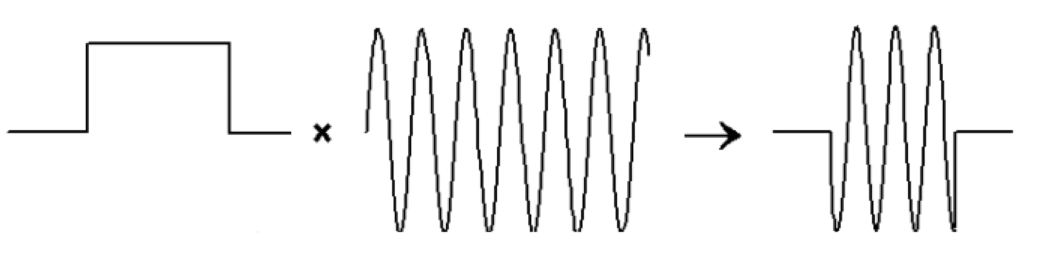
The duration of one pulse is typically many optical cycles, while the duration of measurement can range from nanoseconds to milliseconds or longer. We can often separate the electric field into a slowly-varying envelope $\mathbf{A}(\mathbf{r},t)$, and a fast oscillation at the carrier frequency ${\omega }_0$:

This is depicted in the next figure. The overall pulse shape (left box-like behaviour in the example) is captured by the slowly-varying envelope $\mathbf{A}(\mathbf{r},t),$ while the fast (second, right) oscillation is captured by the $e^{i{\omega }_{0}t}$ term:

Let us next explicitly calculate the instantaneous Poynting vector for such fields. If we define the complex envelopes $\tilde{\mathbf{E}}(\mathbf{r},t)$ and $\tilde{\mathbf{H}}(\mathbf{r},t)$ such that the physical fields are ${\mathbf{E}}_{\text{phys}}=\mathfrak{Re}[\tilde{\mathbf{E}}(\mathbf{r},t)e^{i{\omega }_{0}t}]$ and ${\mathbf{H}}_{\text{phys}}=\mathfrak{Re}[\tilde{\mathbf{H}}(\mathbf{r},t)e^{i{\omega }_{0}t}]$ (where $\tilde{\mathbf{E}}$ and $\tilde{\mathbf{H}}$ are the slowly varying complex amplitudes):

The first term is slowly varying, while the second term oscillates rapidly at $2{\omega }_0$. Therefore, the Poynting vector has slowly varying contributions which change over timescales of the pulse envelope, and fast contributions changing over timescales of the optical cycle (through $2{\omega }_0$).

To obtain a measure for the average energy flux over a measurement time interval $T_m\gg T_0$, we calculate

If $T_m$ is much longer than the optical period $T_0=2\pi /{\omega }_0$, the fast oscillating terms (at $2{\omega }_0$) average to zero over $T_m$. Thus, if the envelopes $\tilde{\mathbf{E}}$ and $\tilde{\mathbf{H}}$ are approximately constant over $T_m$ (or $T_m$ is chosen as an integer multiple of optical periods and envelopes vary slowly within $T_m$), only the slowly-varying term contributes significantly to the average:

For stationary, monochromatic fields, the complex amplitudes $\tilde{\mathbf{E}}(\mathbf{r})$ and $\tilde{\mathbf{H}}(\mathbf{r})$ are independent of time (the envelope is constant). The time-averaged Poynting vector is then

This time-averaged Poynting vector is often used to define the optical intensity $I$:

The intensity is therefore the magnitude of the time-averaged Poynting vector, and its units are typically Watts per square metre (W/m${}^2$) or Watts per square centimetre (W/cm${}^2$). By measuring intensity, we average over the fast varying optical cycle, and thus typically discard direct phase information of the optical field.

1.10 Momentum of Light

Light carries not only energy but also momentum. The momentum density of an electromagnetic field in a medium with refractive index $n$ is $\mathbf{g}=\mathbf{S}/v_p^2=n^2\mathbf{S}/c^2$. The total momentum ${\mathbf{p}}_{\text{field}}$ contained in a volume is ${\int }_V\mathbf{g}dV$.
When light is absorbed or reflected by an object, it exerts a force (radiation pressure) due to the transfer of momentum.

The momentum $\mathrm{\Delta }\mathbf{p}$ transferred to an object that completely absorbs an incident light pulse of energy $U_{pulse}$ propagating in a medium of refractive index $n$ is $\mathrm{\Delta }\mathbf{p}=(U_{pulse}/c)n\hat{\mathbf{k}}$, where $\hat{\mathbf{k}}$ is the direction of light propagation.
For a light beam with time-averaged Poynting vector $⟨\mathbf{S}⟩$ (intensity $I=|⟨\mathbf{S}⟩|$) normally incident on a perfectly absorbing surface of area $A$ for a duration $\mathrm{\Delta }t$, the total energy incident is $U=IA\mathrm{\Delta }t$. The momentum transferred is:

If the surface is inclined such that its normal makes an angle $\theta$ with the incident Poynting vector $⟨\mathbf{S}⟩$, the projected area normal to the beam is $A_{\perp }=A\cos \theta$. The energy incident on area $A$ is $IA\cos \theta \mathrm{\Delta }t$. Thus, the magnitude of momentum transferred to a perfectly absorbing disk is:

where $I_0$ is the incident intensity.

The linear momentum of light finds applications such as in laser cooling and trapping of atoms, optical tweezers, and proposals for light sails for spacecraft. The force exerted is the radiation pressure. For example, for a high-power ultrafast laser with pulse duration $10\text{fs}$, $10\text{PW}$ peak power, and an intensity of ${10}^{23}{\text{W/cm}}^2$, the radiation pressure $P_{\text{rad}}=I/c$ (for normal incidence, perfect absorption in vacuum) can be immense, $P_{\text{rad}}\approx ({10}^{23}\times {10}^4{\text{W/m}}^2)/(3\times {10}^8\text{m/s})\approx 3.3\times {10}^{18}\text{Pa}$, which is about $3\times {10}^{13}$ bar.